2. Discretization Strategy
\( \let\b=\mathbf \)2.1. Literature on DG for Fluid Flow
How to discretize the conservation equations with DG, including how to handle the required fluxes, particularly in the viscous setting, is a current topic of research and internal discussion. The following references are useful:
“The DG Book:” Nodal Discontinuous Galerkin Methods, [Hesthaven_2008]
The BR1 method for discretization of Navier-Stokes, [Bassi_1997]
NS with reactions, [Ihme_2014], and [Cook_2009]
The BR2 method, [Bassi_2000]
Shock handling [Woodward_1984]
Artificial viscosity [Persson_2012]
Boundary Condtitions [Mengaldo_2014], and [Poinsot_1992]
Phenolics modeling [Lachaud_2014]
MIRGE-Com currently employs a strategy akin to the BR1 algorithm outlined in [Bassi_1997], but with thermal terms and chemical reaction sources as outlined in [Ihme_2014] and [Cook_2009].
2.3. Numerical fluxes
Numerical fluxes are responsible for calculating the fluxes at the DG element boundaries. Numerical fluxes must account for the discontinuities at element faces, and calculate a single valued flux that both elements agree on. That is, they must be functions of both \(\pm\) states, and must produce a consistent flux.
For a conservation law \(\frac{\partial \b{Q}}{\partial t} + \nabla \cdot \b{F}(\b{Q}) = \b{S}\), the numerical flux \(h\) must satisfy the consistency relations
2.3.1. Inviscid numerical flux
Approximate and exact Riemann solvers are typically used for inviscid numerical flux functions, \(h_e(\b{Q}_h^+, \b{Q}^-_h; \b{n})\). Typical choices include, but are not limited to:
Local Lax-Friedrichs or Rusanov (LFR)
Harten-Lax-van Leer (HLL)
Roe
Engquist-Osher
MIRGE-Com currently has LFR, and HLL numerical fluxes available from
the inviscid module.
The LFR numerical flux is implemented by inviscid_facial_flux_rusanov() as follows:
where \(\lambda\) is the characteristic max wave-speed of the fluid. Numerical fluxes which penalize the ‘’jump’’ of the state \(\left(\b{Q}_h^+ - \b{Q}_h^-\right) \b{n}\) act as an additional source of dissipation, which has a stabilizing effect on the numerics.
The HLL numerical flux is implemented by inviscid_facial_flux_hll() as follows:
2.3.2. Numerical Fluxes for Viscous Terms
Typically, the Riemann solvers used for inviscid fluxes are not employed for the viscous fluxes of compressible Navier-Stokes equations and the auxiliary equation, \(\b{h}_v\), and \(\b{H}_s\).
The following sections describe the numerical flux functions used for the divergence of the viscous transport flux and the gradient of the solution in the auxiliary equation.
2.3.2.1. Viscous numerical flux
The numerical flux function for the divergence of the viscous transport flux
of the Navier-Stokes equations, \(\b{h}_v\), is implemented in
viscous_facial_flux_central() as follows:
where \(\b{F}^V_{\pm} \equiv \b{F}^V(\b{Q}_h^{\pm}, \b{\Sigma}_h^{\pm})\), is the viscous flux function computed for the (\(\pm\)) sides of the element boundary, respectively.
2.3.2.2. Gradient numerical flux
The available numerical flux functions used for the gradient of the fluid solution,
\(\b{H}_s\), uses num_flux_central() as follows:
2.4. Domain boundary treatments
What happens when \(\partial E \cap \partial\Omega \neq \emptyset\)?
In DG, fluxes are responsible for handling the flow of information between adjacent cells, and for transferring the boundary conditions into the domain from the domain boundary. In DG the boundary conditions boundary conditions are enforced weakly through the fluxes used at the domain boundary faces.
Boundary treatments in MIRGE-Com follow the prescriptions of the the so-called BR1 method descibed by [Bassi_1997], and the boundary treatment strategies outlined by [Mengaldo_2014].
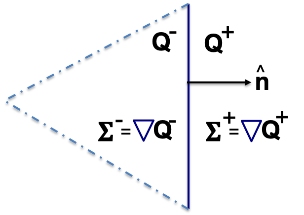
The relevant quantities for the boundary treatments are as follows:
- \(\b{Q}^{\pm}:\):
Conserved quantities on the exterior/interior of the boundary face
- \(\b{Q}_{bc}:\):
Boundary condition for the fluid conserved quantities
- \(\b{\Sigma}^{\pm}:\):
Gradient of conserved quantities on ext/int of boundary face
- \(\b{\Sigma}_{bc}:\):
Boundary condition for gradient of the conserved quantities
- \(\b{v}^{\pm}:\):
Flow velocity on the exterior/interior of boundary face
- \(h^*_e:\):
Boundary facial flux for the divergence of the inviscid flux
- \(h^*_v:\):
Boundary facial flux for divergence of viscous flux
- \(\b{H}_s^*:\):
Boundary flux vector for the gradient of the conserved quantities
- \(\hat{\b{n}}:\):
Outward pointing unit normal for the boundary face
For all \(\partial E \cap \partial\Omega\) the \(+\) side is on the domain boundary. Boundary conditions (\(\b{Q}_{bc}, \b{\Sigma}_{bc}\)) are set by prescribing one or more components of the solution or its gradient on the (+) side of the boundary, (\(\b{Q}^+, \b{\Sigma}^+\)), respectively, or by prescribing one or more components of the boundary fluxes \(h^*_e\), \(h^*_v\), and \(\b{H}^*_s\). Descriptions of particular boundary treatments follow in the next few sections.
2.4.1. Adiabatic slip wall
The slip wall condition is a symmetry condition in which the velocity of the fluid in the direction of the wall normal vanishes. That is:
with fluid velocity \(\b{v}_{fluid}\), wall velocity \(\b{v}_{wall}\), and outward pointing unit normal \(\hat{\b{n}}\). For a fixed wall, \(\b{v}_{fluid} \cdot \hat{\b{n}} = 0\). The components of the fluid velocity in the plane of the wall are left unperturbed by the wall.
More specifically, for the fixed wall in MIRGE-Com, the fluid solution corresponding to this boundary condition is this:
where \(\mathbf{v}_b = \mathbf{v}^{-} - (\mathbf{v}^{-}\cdot\hat{\mathbf{n}})\hat{\mathbf{n}}\).
In MIRGE-Com, this boundary condition is transmitted to the boundary element through the approximate Riemann solver, or numerical flux function, \(h_e(\b{Q}^-, \b{Q}^+)\). As such, the boundary treatment in MIRGE-Com is to prescribe the boundary solution \(\b{Q}^+\) to be used in the numerical flux function to induce the desired boundary condition, \(\b{Q}_{bc}\).
The adiabatic slip wall boundary treatment is implemented by the
AdiabaticSlipBoundary. The boundary solution
is prescribed as follows:
where \(\mathbf{v}^{+} = \mathbf{v}^{-} - 2(\mathbf{v}^{-}\cdot\hat{\mathbf{n}})\hat{\mathbf{n}}\). Note that the boundary solution, \(\b{Q}^+\) is set such that \(\frac{1}{2}(\b{Q}^- + \b{Q}^+) = \b{Q}_{bc}\). When using a Riemann solver to transmit the boundary condition to the boundary element, it is important that the (\(\pm\)) state inputs to the solver result in an intermediate state in which the normal components of velocity vanish.
2.4.1.1. Inviscid fluxes (advection terms)
The flux for the divergence of the inviscid flux is then calculated with the same numerical flux function as used in the volume: \(h^*_e = h_{e}(\b{Q}^-, \b{Q}^+)\).
In practice, when the fluid operators in inviscid, euler,
and navierstokes, go to calculate the flux for the divergence of the
inviscid physical transport fluxes, they call the
inviscid_divergence_flux() function, which for this
adiabatic slip boundary, sets the boundary state, \(\b{Q}^+\) by calling
state_plus(), and returns the numerical flux
\({h}^*_e = h_{e}(\b{Q}^-, \b{Q}^+)\).
2.4.1.2. Viscous fluxes (diffusion terms)
The viscous fluxes depend on both the conserved quantities, and their gradient. The gradient of the conserved quantities is obtained in the solution of the auxiliary equations and the boundary condition imposed on that system is \(\b{Q}_{bc}\).
The boundary flux for the gradient of the conserved quantities is computed using the same numerical flux scheme as in the volume:
The solution of the auxiliary equations yields \(\nabla{\b{Q}}^-\), and the gradients for the species fractions \(Y\) and temperature \(T\), are calculated using the product rule:
We enforce no penetration for the species fractions by setting:
We set the heat flux through the wall to zero by setting:
The boundary viscous flux is then calculated using the same flux function as that in the volume by:
2.4.2. Adiabatic No-slip Wall
The no-slip boundary condition essentially means that the fluid velocity at the wall is equal to that of the wall itself:
For fixed walls, this boundary condition is \(\b{v}_{fluid} = 0\). Specifically, this means the fluid state at the wall for this boundary condition is as follows:
In MIRGE-Com, the no-slip boundary condition is enforced indirectly by providing the fluxes at the element boundaries that correspond to the given boundary condition. For inviscid fluxes, the numerical flux functions are used with a prescribed boundary state to get the fluxes. For the viscous fluxes and for the auxilary equation (i.e. the gradient of the fluid solution), the fluxes are calculated using a prescribed boundary state that is distinct from the one used for the inviscid flux.
The following sections describe both the boundary solutions, and the flux functions used for each step in computing the boundary fluxes for an adiabatic no-slip wall.
2.4.2.1. Inviscid fluxes
For the inviscid fluxes, following [Mengaldo_2014], Step 1 is to prescribe \(\b{Q}^+\) at the wall and Step 2. is to use the approximate Riemann solver (i.e. the numerical flux function, \(h_e\)) to provide the element flux for the divergence operator.
In this section the boundary state, \(\b{Q}^+\), used for each no-slip wall is described. Specifically, we have adiabatic no-slip wall in Step 1a, and an isothermal no-slip wall in Step 1b. Then the numerical flux calculation is described in Step 2.
2.4.2.1.1. Step 1 \(\b{Q}^+\) for adiabatic no-slip
For walls enforcing an adiabatic no-slip condition, the boundary state we use for \(\b{Q}^+\) is as follows:
where \(\b{v}^-\) is the fluid velocity corresponding to \(\b{Q}^-\). Explicity, for our particular equations in MIRGE-Com, we set:
which is just the interior fluid state except with the opposite momentum. This ensures that any Riemann solver used at the boundary will have an intermediate state with 0 velocities on the boundary. Other choices here will lead to non-zero velocities at the boundary, leading to material penetration at the wall; a non-physical result.
Note
For the adiabatic state, the wall temperature is simply taken from the interior solution and we use the interior temperature, \({T}_{in}\). This choice means the difference in total energy between the \((\pm)\) states vanishes and \((\rho{E})^+ = (\rho{E})^-\).
2.4.2.1.2. Step 1b. \(\b{Q}^+\) for isothermal no-slip
For walls enforcing an isothermal no-slip condition, the boundary state we use for \(\b{Q}^+\) is calculated from \(\b{Q}^-\) with a temperature prescribed by the wall temperature, \({T}_{wall}\).
2.4.2.1.3. Step 2. Boundary flux, \({h}^*_e\), for divergence of inviscid flux
The inviscid boundary flux is then calculated from the same numerical flux function used for inviscid interfacial fluxes in the volume:
Intuitively, we expect \(h^*_e\) is equal to the (interior; - side) pressure contribution of \(\b{F}^I(\b{Q}_{bc})\cdot\hat{\b{n}}\) (since \(\b{V}\cdot\hat{\b{n}} = 0\)).
2.4.2.2. Viscous fluxes
MIRGE-Com has a departure from BR1 for the computation of viscous fluxes. This section will describe the viscous flux calculations prescribed by [Bassi_1997], and [Mengaldo_2014], and also what MIRGE-Com is currently doing.
Note
[Mengaldo_2014] prescribes that when computing the gradients of the solution (i.e. the auxiliary equation) and the viscous fluxes, one should use a \(\b{Q}_{bc}\) that is distinct from that used for the advective terms. This reference recommends explicitly setting the boundary velocities to zero for the \(\b{Q}_{bc}\) used in computing \(\nabla{\b{Q}}\) and \(\b{F}_v(\b{Q}_{bc})\).
BR1 and Mengaldo prescribe the following boundary treatment:
The viscous boundary flux at solid walls is computed as:
where \(\b{Q}_{bc}\) are the same values used to prescribe \(h^*_e\).
If there are no conditions on \(\nabla\b{Q}\cdot\hat{\b{n}}\), then:
MIRGE-Com currently does the following:
where \(\b{Q}_{bc}\) are the same values used to prescribe \(h^*_e\).
In MIRGE-Com, we use the central flux to transfer viscous BCs to the domain:
2.4.2.2.1. Gradient boundary flux
The boundary flux for \(\nabla{\b{Q}}\) (i.e. for the auxiliary at the boundary is computed with a central flux as follows:
using the no-slip boundary solution, \(\b{Q}_{bc}\), as defined above. The note above about [Mengaldo_2014] using a distinct \(\b{Q}_{bc}\) is relevant here.
Since:
We compute \(\nabla{Y}\) and \(\nabla{E}\) from the product rule:
2.4.2.3. Inflow/outflow boundaries
2.4.2.3.1. Inviscid boundary flux
2.4.2.3.2. Viscous boundary flux
2.4.2.3.3. Gradient boundary flux
\(\b{Q}_{bc}\) is also used to define the gradient boundary flux: