4.4. Gas Dynamics
mirgecom.fluid provides common utilities for fluid simulation.
4.4.1. Conserved Quantities Handling
- class mirgecom.fluid.ConservedVars(mass, energy, momentum, species_mass=<factory>)[source]
Store and resolve quantities according to the fluid conservation equations.
Store and resolve quantities that correspond to the fluid conservation equations for the canonical conserved quantities (mass, energy, momentum, and species masses) per unit volume: \((\rho,\rho{E},\rho\vec{V}, \rho{Y_s})\) from an agglomerated object array. This data structure is intimately related to the helper function
make_conserved()which forms CV objects from flat object array representations of the data.- dim
Integer indicating spatial dimension of the simulation
- mass
DOFArrayfor scalars or object array ofDOFArrayfor vector quantities corresponding to the mass continuity equation.
- energy
DOFArrayfor scalars or object array ofDOFArrayfor vector quantities corresponding to the energy conservation equation.
- momentum
Object array (
numpy.ndarray) with shape(ndim,)ofDOFArray, or an object array with shape(ndim, ndim)respectively for scalar or vector quantities corresponding to the ndim equations of momentum conservation.
- species_mass
Object array (
numpy.ndarray) with shape(nspecies,)ofDOFArray, or an object array with shape(nspecies, ndim)respectively for scalar or vector quantities corresponding to the nspecies species mass conservation equations.
- Example::
Use ConservedVars to access the fluid conserved variables (CV).
The vector of fluid CV is commonly denoted as \(\mathbf{Q}\), and for a fluid mixture with nspecies species and in ndim spatial dimensions takes the form:
\[\begin{split}\mathbf{Q} &= \begin{bmatrix}\rho\\\rho{E}\\\rho{v}_{i}\\\rho{Y}_{\alpha}\end{bmatrix},\end{split}\]with the ndim-vector components of fluid velocity (\(v_i\)), and the nspecies-vector of species mass fractions (\(Y_\alpha\)). In total, the fluid system has \(N_{\text{eq}}\) = (ndim + 2 + nspecies) equations.
Internally to MIRGE-Com, \(\mathbf{Q}\) is stored as an object array (
numpy.ndarray) ofDOFArray, one for each component of the fluid \(\mathbf{Q}\), i.e. a flat object array of \(N_{\text{eq}}\)DOFArray.To use this dataclass for a fluid CV-specific view on the content of \(\mathbf{Q}\), one can call
make_conserved()to get a ConservedVars dataclass object that resolves the fluid CV associated with each conservation equation:fluid_cv = make_conserved(dim=ndim, q=Q),
after which:
fluid_mass_density = fluid_cv.mass  # a DOFArray with fluid density
fluid_momentum_density = fluid_cv.momentum  # ndim-vector obj array
fluid_species_mass_density = fluid_cv.species_mass  # nspecies-vector
Examples of using ConservedVars as in this example can be found in:
- Example::
Use join to create an agglomerated \(\mathbf{Q}\) array from the fluid conserved quantities (CV).
See the first example for the definition of CV, \(\mathbf{Q}\), ndim, nspecies, and \(N_{\text{eq}}\).
Often, a user starts with the fluid conserved quantities like mass and energy densities, and it is desired to glom those quantities together into a MIRGE-compatible \(\mathbf{Q}\) data structure.
For example, a solution initialization routine may set the fluid quantities:
rho = ... # rho is a DOFArray with fluid density
v = ... # v is an ndim-vector of DOFArray with components of velocity
e = ... # e is a DOFArray with fluid energy
An agglomerated array of fluid independent variables can then be created with:
q = cv.join()
after which q will be an obj array of \(N_{\text{eq}}\) DOFArrays containing the fluid conserved state data.
Examples of this sort of use for join can be found in:
- Example::
Use ConservedVars to access a vector quantity for each fluid equation.
See the first example for the definition of CV, \(\mathbf{Q}\), ndim, nspecies, and \(N_{\text{eq}}\).
Suppose the user wants to access the gradient of the fluid state, \(\nabla\mathbf{Q}\), in a fluid-specific way. For a fluid \(\mathbf{Q}\), such an object would be:
\[\begin{split}\nabla\mathbf{Q} &= \begin{bmatrix}(\nabla\rho)_j\\(\nabla\rho{E})_j\\(\nabla\rho{v}_{i})_j \\(\nabla\rho{Y}_{\alpha})_j\end{bmatrix},\end{split}\]where \(1 \le j \le \text{ndim}\), such that the first component of \(\mathbf{Q}\) is an ndim-vector corresponding to the gradient of the fluid density, i.e. object array of ndim DOFArray. Similarly for the energy term. The momentum part of \(\nabla\mathbf{Q}\) is a 2D array with shape
(ndim, ndim)with each row corresponding to the gradient of a component of the ndim-vector of fluid momentum. The species portion of \(\nabla\mathbf{Q}\) is a 2D array with shape(nspecies, ndim)with each row being the gradient of a component of the nspecies-vector corresponding to the species mass.Presuming that grad_q is the agglomerated MIRGE data structure with the gradient data, this dataclass can be used to get a fluid CV-specific view on the content of \(\nabla\mathbf{Q}\). One can call
make_conserved()to get a ConservedVars dataclass object that resolves the vector quantity associated with each conservation equation:grad_q = gradient_operator(discr, q) grad_cv = make_conserved(ndim, q=grad_q),
after which:
grad_mass = grad_cv.mass  # an `ndim`-vector grad(fluid density)
grad_momentum = grad_cv.momentum  # 2D array shape=(ndim, ndim)
grad_spec = grad_cv.species_mass  # 2D (nspecies, ndim)
Examples of this type of use for ConservedVars can be found in:
- Parameters:
- mirgecom.fluid.make_conserved(dim, mass=None, energy=None, momentum=None, species_mass=None, q=None, scalar_quantities=None, vector_quantities=None)[source]
Create
ConservedVarsfrom separated conserved quantities.
4.4.2. Helper Functions
- mirgecom.fluid.velocity_gradient(cv, grad_cv)[source]
Compute the gradient of fluid velocity.
Computes the gradient of fluid velocity from:
\[\nabla{v_i} = \frac{1}{\rho}(\nabla(\rho{v_i})-v_i\nabla{\rho}),\]where \(v_i\) is ith velocity component.
Note
The product rule is used to evaluate gradients of the primitive variables from the existing data of the gradient of the fluid solution, \(\nabla\mathbf{Q}\), following [Hesthaven_2008], section 7.5.2. If something like BR1 ([Bassi_1997]) is done to treat the viscous terms, then \(\nabla{\mathbf{Q}}\) should be naturally available.
Some advantages of doing it this way:
avoids an additional DG gradient computation
enables the use of a quadrature discretization for computation
jibes with the already-applied bcs of \(\mathbf{Q}\)
- Parameters:
cv (ConservedVars) – the fluid conserved variables
grad_cv (ConservedVars) – the gradients of the fluid conserved variables
- Returns:
object array of
DOFArrayfor each row of \(\partial_j{v_i}\). e.g. for 2D: \(\left( \begin{array}{cc} \partial_{x}\mathbf{v}_{x}&\partial_{y}\mathbf{v}_{x} \\ \partial_{x}\mathbf{v}_{y}&\partial_{y}\mathbf{v}_{y} \end{array} \right)\)- Return type:
- mirgecom.fluid.species_mass_fraction_gradient(cv, grad_cv)[source]
Compute the gradient of species mass fractions.
Computes the gradient of species mass fractions from:
\[\nabla{Y}_{\alpha} = \frac{1}{\rho}\left(\nabla(\rho{Y}_{\alpha})-{Y_\alpha}(\nabla{\rho})\right),\]where \({Y}_{\alpha}\) is the mass fraction for species \({\alpha}\).
- Parameters:
cv (ConservedVars) – the fluid conserved variables
grad_cv (ConservedVars) – the gradients of the fluid conserved variables
- Returns:
object array of
DOFArrayrepresenting \(\partial_j{Y}_{\alpha}\).- Return type:
mirgecom.eos provides implementations of gas equations of state.
4.4.3. Equations of State
This module is designed provide Equation of State objects used to compute and manage the relationships between and among state and thermodynamic variables.
- class mirgecom.eos.GasDependentVars(temperature, pressure, speed_of_sound, smoothness_mu, smoothness_kappa, smoothness_d, smoothness_beta)[source]
State-dependent quantities for
GasEOS.Prefer individual methods for model use, use this structure for visualization or probing.
- Parameters:
- temperature
- pressure
- speed_of_sound
- smoothness_mu
- smoothness_kappa
- smoothness_beta
- smoothness_d
- class mirgecom.eos.MixtureDependentVars(temperature, pressure, speed_of_sound, smoothness_mu, smoothness_kappa, smoothness_d, smoothness_beta, species_enthalpies)[source]
Mixture state-dependent quantities for
MixtureEOS...attribute:: species_enthalpies
- class mirgecom.eos.GasEOS[source]
Abstract interface to equation of state class.
Equation of state (EOS) classes are responsible for computing relations between fluid or gas state variables.
Each interface call takes an
ConservedVarsobject array representing the simulation state quantities. Each EOS class implementation should document its own state data requirements.- abstractmethod pressure(cv, temperature)[source]
Get the gas pressure.
- Parameters:
cv (ConservedVars)
temperature (DOFArray)
- abstractmethod temperature(cv, temperature_seed=None)[source]
Get the gas temperature.
- Parameters:
cv (ConservedVars)
temperature_seed (DOFArray | None)
- Return type:
- abstractmethod sound_speed(cv, temperature)[source]
Get the gas sound speed.
- Parameters:
cv (ConservedVars)
temperature (DOFArray)
- abstractmethod internal_energy(cv)[source]
Get the thermal energy of the gas.
- Parameters:
cv (ConservedVars)
- abstractmethod gas_const(cv=None, temperature=None, species_mass_fractions=None)[source]
Get the specific gas constant (\(R_s\)).
- Parameters:
cv (ConservedVars | None)
temperature (DOFArray | None)
species_mass_fractions (ndarray | None)
- Return type:
- dependent_vars(cv, temperature_seed=None, smoothness_mu=None, smoothness_kappa=None, smoothness_d=None, smoothness_beta=None)[source]
Get an agglomerated array of the dependent variables.
Certain implementations of
GasEOS(e.g.MixtureEOS) may raiseTemperatureSeedMissingErrorif temperature_seed is not given.- Parameters:
- Return type:
- abstractmethod total_energy(cv, pressure, temperature)[source]
Get the total (thermal + kinetic) energy for the gas.
- Parameters:
cv (ConservedVars)
pressure (DOFArray)
temperature (DOFArray)
- abstractmethod kinetic_energy(cv)[source]
Get the kinetic energy for the gas.
- Parameters:
cv (ConservedVars)
- abstractmethod gamma(cv=None, temperature=None)[source]
Get the ratio of gas specific heats Cp/Cv.
- Parameters:
cv (ConservedVars | None)
temperature (DOFArray | None)
- class mirgecom.eos.MixtureEOS[source]
Abstract interface to gas mixture equation of state class.
This EOS base class extends the GasEOS base class to include the necessary interface for dealing with gas mixtures.
- abstractmethod get_density(pressure, temperature, species_mass_fractions)[source]
Get the density from pressure, temperature, and species fractions (Y).
- abstractmethod get_production_rates(cv, temperature)[source]
Get the production rate for each species.
- Parameters:
cv (ConservedVars)
temperature (DOFArray)
- abstractmethod species_enthalpies(cv, temperature)[source]
Get the species specific enthalpies.
- Parameters:
cv (ConservedVars)
temperature (DOFArray)
- abstractmethod get_species_source_terms(cv, temperature)[source]
Get the species mass source terms to be used on the RHS for chemistry.
- Parameters:
cv (ConservedVars)
temperature (DOFArray)
- abstractmethod get_temperature_seed(ary=None, temperature_seed=None)[source]
Get a constant and uniform guess for the gas temperature.
This function returns an appropriately sized DOFArray for the temperature field that will be used as a starting point for the solve to find the actual temperature field of the gas.
- class mirgecom.eos.IdealSingleGas(gamma=1.4, gas_const=287.1)[source]
Ideal gas law single-component gas (\(p = \rho{R}{T}\)).
The specific gas constant, R, defaults to the air-like 287.1 J/(kg*K), but can be set according to simulation units and materials.
Each interface call expects that the
ConservedVarsobject representing the simulation conserved quantities contains at least the canonical conserved quantities mass (\(\rho\)), energy (\(\rho{E}\)), and momentum (\(\rho\vec{V}\)).- gamma(cv=None, temperature=None)[source]
Get specific heat ratio Cp/Cv.
- Parameters:
cv (
ConservedVars) – Unused for this EOStemperature (
DOFArray) – Unused for this EOS
- Return type:
- heat_capacity_cp(cv=None, temperature=None)[source]
Get specific heat capacity at constant pressure (\(C_p\)).
- Parameters:
cv (
ConservedVars) – Unused for this EOStemperature (
DOFArray) – Unused for this EOS
- Return type:
- heat_capacity_cv(cv=None, temperature=None)[source]
Get specific heat capacity at constant volume (\(C_v\)).
- Parameters:
cv (
ConservedVars) – Unused for this EOStemperature (
DOFArray) – Unused for this EOS
- Return type:
- gas_const(cv=None, temperature=None, species_mass_fractions=None)[source]
Get specific gas constant R.
- Parameters:
cv (
ConservedVars) – Unused for this EOStemperature (
DOFArray) – Unused for this EOSspecies_mass_fractions (numpy.ndarray) – Unused for this EOS
- Return type:
- get_density(pressure, temperature, species_mass_fractions=None)[source]
Get gas density from pressure and temperature.
The gas density is calculated as:
\[\rho = \frac{p}{R_s T}\]- Parameters:
species_mass_fractions (numpy.ndarray) – Unused for this EOS
pressure (DOFArray)
temperature (DOFArray)
- Return type:
- kinetic_energy(cv)[source]
Get kinetic energy of gas.
The kinetic energy is calculated as:
\[k = \frac{1}{2\rho}(\rho\vec{V} \cdot \rho\vec{V})\]- Parameters:
cv (ConservedVars)
- Return type:
- internal_energy(cv)[source]
Get internal thermal energy of gas.
The internal energy (e) is calculated as:
\[e = \rho{E} - \frac{1}{2\rho}(\rho\vec{V} \cdot \rho\vec{V})\]- Parameters:
cv (ConservedVars)
- Return type:
- pressure(cv, temperature=None)[source]
Get thermodynamic pressure of the gas.
Gas pressure (p) is calculated from the internal energy (e) as:
\[p = (\gamma - 1)e\]- Parameters:
temperature (
DOFArray) – Unused for this EOScv (ConservedVars)
- Return type:
- sound_speed(cv, temperature=None)[source]
Get the speed of sound in the gas.
The speed of sound (c) is calculated as:
\[c = \sqrt{\frac{\gamma{p}}{\rho}}\]- Parameters:
temperature (
DOFArray) – Unused for this EOScv (ConservedVars)
- Return type:
- temperature(cv, temperature_seed=None)[source]
Get the thermodynamic temperature of the gas.
The thermodynamic temperature (T) is calculated from the internal energy (e) and specific gas constant (R) as:
\[T = \frac{(\gamma - 1)e}{R\rho}\]- Parameters:
temperature_seed (float or
DOFArray) – Unused for this EOS.cv (ConservedVars)
- Return type:
- total_energy(cv, pressure, temperature=None)[source]
Get gas total energy from mass, pressure, and momentum.
The total energy density (rhoE) is calculated from the mass density (rho) , pressure (p) , and momentum (rhoV) as:
\[\rho{E} = \frac{p}{(\gamma - 1)} + \frac{1}{2}\rho(\vec{v} \cdot \vec{v})\]Note
The total_energy function computes cv.energy from pressure, mass, and momentum in this case. In general in the EOS we need DV = EOS(CV), and inversions CV = EOS(DV). This is one of those inversion interfaces.
- Parameters:
cv (
ConservedVars) – The conserved variablespressure (
DOFArray) – The fluid pressuretemperature (
DOFArray) – Unused for this EOS
- Returns:
The total energy of the fluid (i.e. internal + kinetic)
- Return type:
- get_internal_energy(temperature, species_mass_fractions=None)[source]
Get the gas thermal energy from temperature.
The gas internal energy \(e\) is calculated from:
\[e = \frac{R_s T}{\left(\gamma - 1\right)}\]
- dependent_vars(cv, temperature_seed=None, smoothness_mu=None, smoothness_kappa=None, smoothness_d=None, smoothness_beta=None)
Get an agglomerated array of the dependent variables.
Certain implementations of
GasEOS(e.g.MixtureEOS) may raiseTemperatureSeedMissingErrorif temperature_seed is not given.- Parameters:
- Return type:
- class mirgecom.eos.PyrometheusMixture(pyrometheus_mech, temperature_guess=300.0)[source]
Ideal gas mixture (\(p = \rho{R}_\mathtt{mix}{T}\)).
This is the
pyrometheus-based EOS. Please refer to thedocumentation of Pyrometheusfor underlying implementation details.Each interface call expects that the
mirgecom.fluid.ConservedVarsobject representing the simulation conserved quantities contains at least the canonical conserved quantities mass (\(\rho\)), energy (\(\rho{E}\)), and momentum (\(\rho\vec{V}\)), and the vector of species masses, (\(\rho{Y}_\alpha\)).Important
When using this EOS, users should take care to match solution initialization with the appropriate units that are used in the user-provided Cantera mechanism input files.
- __init__(pyrometheus_mech, temperature_guess=300.0)[source]
Initialize Pyrometheus-based EOS with mechanism class.
- Parameters:
pyrometheus_mech (
Thermochemistry) – ThepyrometheusmechanismThermochemistryobject that is generated by the user with a call to pyrometheus.get_thermochem_class. To create the mechanism object, users need to provide a mechanism input file. Several example mechanisms are provided in mirgecom/mechanisms/ and can be used through themirgecom.mechanisms.get_mechanism_input().tguess (float) – This provides a constant starting temperature for the Newton iterations used to find the mixture temperature. It defaults to 300.0 Kelvin. This parameter is important for the performance and proper function of the code. Users should set a tguess that is close to the average temperature of the simulated domain.
- pressure(cv, temperature)[source]
Get thermodynamic pressure of the gas.
Gas pressure (\(p\)) is calculated using ideal gas law:
\[p = \rho R_{mix} T\]- Parameters:
cv (ConservedVars)
temperature (DOFArray)
- Return type:
- temperature(cv, temperature_seed=None)[source]
Get the thermodynamic temperature of the gas.
The thermodynamic temperature (\(T\)) is calculated iteratively with Newton-Raphson method from the mixture internal energy (\(e\)) as:
\[e(T) = \sum_i e_i(T) Y_i\]- Parameters:
temperature_seed (float or
DOFArray) – Data from which to seed temperature calculation.cv (ConservedVars)
- Return type:
- sound_speed(cv, temperature)[source]
Get the speed of sound in the gas.
The speed of sound (\(c\)) is calculated as:
\[c = \sqrt{\frac{\gamma_{\mathtt{mix}}{p}}{\rho}}\]- Parameters:
cv (ConservedVars)
temperature (DOFArray)
- Return type:
- internal_energy(cv)[source]
Get internal thermal energy of gas.
The internal energy (\(e\)) is calculated as:
\[e = \rho{E} - \frac{1}{2\rho}(\rho\vec{V} \cdot \rho\vec{V})\]- Parameters:
cv (ConservedVars)
- Return type:
- gas_const(cv=None, temperature=None, species_mass_fractions=None)[source]
Get specific gas constant \(R_s\).
The mixture specific gas constant is calculated as
\[R_s = \frac{R}{\sum{\frac{{Y}_\alpha}{{M}_\alpha}}}\]by the
pyrometheusmechanism provided by the user. In this equation, \({M}_\alpha\) are the species molar masses and R is the universal gas constant.- Parameters:
cv (ConservedVars | None)
temperature (DOFArray | None)
species_mass_fractions (ndarray | None)
- Return type:
- dependent_vars(cv, temperature_seed=None, smoothness_mu=None, smoothness_kappa=None, smoothness_d=None, smoothness_beta=None)
Get an agglomerated array of the dependent variables.
Certain implementations of
GasEOS(e.g.MixtureEOS) may raiseTemperatureSeedMissingErrorif temperature_seed is not given.- Parameters:
- Return type:
- total_energy(cv, pressure, temperature)[source]
Get gas total energy from mass, pressure, and momentum.
The total energy density (\(\rho E\)) is calculated from the mass density (\(\rho\)) , pressure (\(p\)) , and momentum (\(\rho\vec{V}\)) as:
\[\rho E = \frac{p}{(\gamma_{\mathtt{mix}} - 1)} + \frac{1}{2}\rho(\vec{v} \cdot \vec{v})\]Note
The total_energy function computes cv.energy from pressure, mass, and momentum in this case. In general in the EOS we need DV = EOS(CV), and inversions CV = EOS(DV). This is one of those inversion interfaces.
- Parameters:
cv (ConservedVars)
pressure (DOFArray)
temperature (DOFArray)
- Return type:
- kinetic_energy(cv)[source]
Get kinetic (i.e. not internal) energy of gas.
The kinetic energy is calculated as:
\[k = \frac{1}{2\rho}(\rho\vec{V} \cdot \rho\vec{V})\]- Parameters:
cv (ConservedVars)
- Return type:
- heat_capacity_cv(cv, temperature)[source]
Get mixture-averaged specific heat capacity at constant volume.
- Parameters:
cv (ConservedVars)
temperature (DOFArray)
- Return type:
- heat_capacity_cp(cv, temperature)[source]
Get mixture-averaged specific heat capacity at constant pressure.
- Parameters:
cv (ConservedVars)
temperature (DOFArray)
- Return type:
- gamma(cv, temperature)[source]
Get mixture-averaged heat capacity ratio, \(\frac{C_p}{C_p - R_s}\).
- Parameters:
cv (ConservedVars)
temperature (DOFArray)
- Return type:
- get_internal_energy(temperature, species_mass_fractions)[source]
Get the gas thermal energy from temperature, and species fractions (Y).
The gas internal energy \(e\) is calculated from:
\[e = R_s T \sum{Y_\alpha e_\alpha}\]
- get_density(pressure, temperature, species_mass_fractions)[source]
Get the density from pressure, temperature, and species fractions (Y).
- get_production_rates(cv, temperature)[source]
Get the chemical production rates for each species.
- Parameters:
cv (ConservedVars)
temperature (DOFArray)
- Return type:
- species_enthalpies(cv, temperature)[source]
Get the species specific enthalpies.
- Parameters:
cv (ConservedVars)
temperature (DOFArray)
- Return type:
- get_species_source_terms(cv, temperature)[source]
Get the species mass source terms to be used on the RHS for chemistry.
- Returns:
Chemistry source terms
- Return type:
- Parameters:
cv (ConservedVars)
temperature (DOFArray)
- get_temperature_seed(ary=None, temperature_seed=None)[source]
Get a cv-shaped array with which to seed temperature calcuation.
- Parameters:
cv (
ConservedVars) –ConservedVarsused to conjure the required shape for the returned temperature guess.temperature_seed (float or
DOFArray) – Optional data from which to seed temperature calculation.ary (DOFArray | None)
- Returns:
The temperature with which to seed the Newton solver in :module:thermochemistry.
- Return type:
4.4.4. Exceptions
mirgecom.transport provides methods/utils for transport properties.
4.4.5. Transport Models
This module is designed provide Transport Model objects used to compute and manage the transport properties in viscous flows. The transport properties currently implemented are the dynamic viscosity (\(\mu\)), the bulk viscosity (\(\mu_{B}\)), the thermal conductivity (\(\kappa\)), and the species diffusivities (\(d_{\alpha}\)).
- class mirgecom.transport.GasTransportVars(bulk_viscosity, viscosity, thermal_conductivity, species_diffusivity)[source]
State-dependent quantities for
TransportModel.Prefer individual methods for model use, use this structure for visualization or probing.
- Parameters:
- bulk_viscosity
- viscosity
- thermal_conductivity
- species_diffusivity
- class mirgecom.transport.TransportModel[source]
Abstract interface to thermo-diffusive transport model class.
Transport model classes are responsible for computing relations between fluid or gas state variables and thermo-diffusive transport properties for those fluids.
- bulk_viscosity(cv, dv=None, eos=None)[source]
Get the bulk viscosity for the gas (\({\mu}_{B}\)).
- Parameters:
cv (ConservedVars)
dv (GasDependentVars | None)
eos (GasEOS | None)
- Return type:
- viscosity(cv, dv=None, eos=None)[source]
Get the gas dynamic viscosity, \(\mu\).
- Parameters:
cv (ConservedVars)
dv (GasDependentVars | None)
eos (GasEOS | None)
- Return type:
- thermal_conductivity(cv, dv=None, eos=None)[source]
Get the gas thermal_conductivity, \(\kappa\).
- Parameters:
cv (ConservedVars)
dv (GasDependentVars | None)
eos (GasEOS | None)
- Return type:
- species_diffusivity(cv, dv=None, eos=None)[source]
Get the vector of species diffusivities, \({d}_{\alpha}\).
- Parameters:
cv (ConservedVars)
dv (GasDependentVars | None)
eos (GasEOS | None)
- Return type:
- volume_viscosity(cv, dv=None, eos=None)[source]
Get the 2nd coefficent of viscosity, \(\lambda\).
- Parameters:
cv (ConservedVars)
dv (GasDependentVars | None)
eos (GasEOS | None)
- Return type:
- transport_vars(cv, dv=None, eos=None)[source]
Compute the transport properties from the conserved state.
- Parameters:
cv (ConservedVars)
dv (GasDependentVars | None)
eos (GasEOS | None)
- Return type:
- class mirgecom.transport.SimpleTransport(bulk_viscosity=0, viscosity=0, thermal_conductivity=0, species_diffusivity=None)[source]
Transport model with uniform, constant properties.
Inherits from (and implements)
TransportModel.- __init__(bulk_viscosity=0, viscosity=0, thermal_conductivity=0, species_diffusivity=None)[source]
Initialize uniform, constant transport properties.
- bulk_viscosity(cv, dv=None, eos=None)[source]
Get the bulk viscosity for the gas, \(\mu_{B}\).
- Parameters:
cv (ConservedVars)
dv (GasDependentVars | None)
eos (GasEOS | None)
- Return type:
- viscosity(cv, dv=None, eos=None)[source]
Get the gas dynamic viscosity, \(\mu\).
- Parameters:
cv (ConservedVars)
dv (GasDependentVars | None)
eos (GasEOS | None)
- Return type:
- volume_viscosity(cv, dv=None, eos=None)[source]
Get the 2nd viscosity coefficent, \(\lambda\).
In this transport model, the second coefficient of viscosity is defined as:
\[\lambda = \left(\mu_{B} - \frac{2\mu}{3}\right)\]- Parameters:
cv (ConservedVars)
dv (GasDependentVars | None)
eos (GasEOS | None)
- Return type:
- thermal_conductivity(cv, dv=None, eos=None)[source]
Get the gas thermal_conductivity, \(\kappa\).
- Parameters:
cv (ConservedVars)
dv (GasDependentVars | None)
eos (GasEOS | None)
- Return type:
- species_diffusivity(cv, dv=None, eos=None)[source]
Get the vector of species diffusivities, \({d}_{\alpha}\).
- Parameters:
cv (ConservedVars)
dv (GasDependentVars | None)
eos (GasEOS | None)
- Return type:
- class mirgecom.transport.PowerLawTransport(alpha=0.6, beta=4.093e-07, sigma=2.5, n=0.666, species_diffusivity=None, lewis=None)[source]
Transport model with simple power law properties.
Inherits from (and implements)
TransportModelbased on a temperature-dependent power law.- __init__(alpha=0.6, beta=4.093e-07, sigma=2.5, n=0.666, species_diffusivity=None, lewis=None)[source]
Initialize power law coefficients and parameters.
- Parameters:
alpha (float) – The bulk viscosity parameter. The default value is “air”.
beta (float) – The dynamic viscosity linear parameter. The default value is “air”.
n (float) – The temperature exponent for dynamic viscosity. The default value is “air”.
sigma (float) – The heat conductivity linear parameter. The default value is “air”.
lewis (numpy.ndarray) – If required, the Lewis number specify the relation between the thermal conductivity and the species diffusivities. The input array must have a shape of “nspecies”.
- bulk_viscosity(cv, dv, eos=None)[source]
Get the bulk viscosity for the gas, \(\mu_{B}\).
\[\mu_{B} = \alpha\mu\]- Parameters:
cv (ConservedVars)
dv (GasDependentVars)
eos (GasEOS | None)
- Return type:
- viscosity(cv, dv, eos=None)[source]
Get the gas dynamic viscosity, \(\mu\).
\(\mu = \beta{T}^n\)
- Parameters:
cv (ConservedVars)
dv (GasDependentVars)
eos (GasEOS | None)
- Return type:
- volume_viscosity(cv, dv, eos=None)[source]
Get the 2nd viscosity coefficent, \(\lambda\).
In this transport model, the second coefficient of viscosity is defined as:
\[\lambda = \left(\alpha - \frac{2}{3}\right)\mu\]- Parameters:
cv (ConservedVars)
dv (GasDependentVars)
eos (GasEOS | None)
- Return type:
- thermal_conductivity(cv, dv, eos)[source]
Get the gas thermal conductivity, \(\kappa\).
\[\kappa = \sigma\mu{C}_{v}\]- Parameters:
cv (ConservedVars)
dv (GasDependentVars)
eos (GasEOS)
- Return type:
- species_diffusivity(cv, dv, eos)[source]
Get the vector of species diffusivities, \({d}_{\alpha}\).
The species diffusivities can be either (1) specified directly or (2) using user-imposed Lewis number \(Le\) w/shape “nspecies”
In the latter, it is then evaluate based on the heat capacity at constant pressure \(C_p\) and the thermal conductivity \(\kappa\) as:
\[d_{\alpha} = \frac{\kappa}{\rho \; Le \; C_p}\]- Parameters:
cv (ConservedVars)
dv (GasDependentVars)
eos (GasEOS)
- Return type:
- class mirgecom.transport.MixtureAveragedTransport(pyrometheus_mech, alpha=0.6, factor=1.0, lewis=None, epsilon=0.0001, singular_diffusivity=1e-06)[source]
Transport model with mixture averaged transport properties.
Inherits from (and implements)
TransportModelbased on a temperature-dependent fit from Pyrometheus/Cantera weighted by the mixture composition. The mixture-averaged rules used follow those discussed in chapter 12 from [Kee_2003].- __init__(pyrometheus_mech, alpha=0.6, factor=1.0, lewis=None, epsilon=0.0001, singular_diffusivity=1e-06)[source]
Initialize mixture averaged transport coefficients and parameters.
- Parameters:
pyrometheus_mech (
Thermochemistry) – ThepyrometheusmechanismThermochemistryobject that is generated by the user with a call to pyrometheus.get_thermochem_class. To create the mechanism object, users need to provide a mechanism input file. Several example mechanisms are provided in mirgecom/mechanisms/ and can be used through themirgecom.mechanisms.get_mechanism_input().alpha (float) – The bulk viscosity parameter. The default value is “air”.
factor (float) – Scaling factor to artifically scale up or down the transport coefficients. The default is to keep the physical value, i.e., 1.0.
lewis (numpy.ndarray) – If required, the Lewis number specify the relation between the thermal conductivity and the species diffusivities. The input array must have a shape of “nspecies”.
epsilon (float) – Parameter to avoid single-species case where \(Y_i \to 1\) that may lead to singular division in the mixture rule. If \(1 - Y_i < \epsilon\), a prescribed diffusivity is used instead. Default to 1e-4.
singular_diffusivity (float) – Diffusivity for the singular case. The actual number should’t matter since, in the single-species case, diffusion is proportional to a nearly zero-gradient. Default to 1e-6 for all species.
- bulk_viscosity(cv, dv, eos=None)[source]
Get the bulk viscosity for the gas, \(\mu_{B}\).
\[\mu_{B} = \alpha\mu\]- Parameters:
cv (ConservedVars)
dv (GasDependentVars)
eos (GasEOS | None)
- Return type:
- viscosity(cv, dv, eos=None)[source]
Get the mixture dynamic viscosity, \(\mu^{(m)}\).
The viscosity depends on the mixture composition given by \(X_k\) mole fraction and pure species viscosity \(\mu_k\) of the individual species. The latter depends on the temperature and it is evaluated by Pyrometheus.
\[\mu^{(m)} = \sum_{k=1}^{K} \frac{X_k \mu_k}{\sum_{j=1}^{K} X_j\phi_{kj}}\]\[\phi_{kj} = \frac{1}{\sqrt{8}} \left( 1 + \frac{W_k}{W_j} \right)^{-\frac{1}{2}} \left( 1 + \left[ \frac{\mu_k}{\mu_j} \right]^{\frac{1}{2}} \left[ \frac{W_j}{W_k} \right]^{\frac{1}{4}} \right)^2\]- Parameters:
cv (ConservedVars)
dv (GasDependentVars)
eos (GasEOS | None)
- Return type:
- volume_viscosity(cv, dv, eos=None)[source]
Get the 2nd viscosity coefficent, \(\lambda\).
In this transport model, the second coefficient of viscosity is defined as:
\[\lambda = \left(\alpha - \frac{2}{3}\right)\mu\]- Parameters:
cv (ConservedVars)
dv (GasDependentVars)
eos (GasEOS | None)
- Return type:
- thermal_conductivity(cv, dv, eos)[source]
Get the gas thermal_conductivity, \(\kappa\).
The thermal conductivity can be obtained from Pyrometheus using a mixture averaged rule considering the species heat conductivities and mole fractions:
\[\kappa = \frac{1}{2} \left( \sum_{k=1}^{K} X_k \lambda_k + \frac{1}{\sum_{k=1}^{K} \frac{X_k}{\lambda_k} }\right)\]- Parameters:
cv (ConservedVars)
dv (GasDependentVars)
eos (GasEOS)
- Return type:
- species_diffusivity(cv, dv, eos)[source]
Get the vector of species diffusivities, \({d}_{i}\).
The species diffusivities can be obtained directly from Pyrometheus using a mixture averaged rule considering the species binary mass diffusivities \(d_{ij}\) and the mass fractions \(Y_i\)
\[d_{i}^{(m)} = \frac{1 - Y_i}{\sum_{j\ne i} \frac{X_j}{d_{ij}}}\]In regions with a single species, the above equation is ill-conditioned and a constant diffusivity is used instead.
The user can prescribe an array with the Lewis number \(Le\) for each species. Then, it is used together with the mixture termal conductivity and the heat capacity at constant pressure \(C_p\) to yield the diffusivity.
\[d_{i} = \frac{\kappa}{\rho \; Le \; C_p}\]- Parameters:
cv (ConservedVars)
dv (GasDependentVars)
eos (GasEOS)
- Return type:
- class mirgecom.transport.ArtificialViscosityTransportDiv(av_mu, av_prandtl, physical_transport=None, av_species_diffusivity=None)[source]
Transport model for add artificial viscosity.
Inherits from (and implements)
TransportModel.Takes a physical transport model and adds the artificial viscosity contribution to it. Defaults to simple transport with inviscid settings. This is equivalent to inviscid flow with artifical viscosity enabled.
- __init__(av_mu, av_prandtl, physical_transport=None, av_species_diffusivity=None)[source]
Initialize uniform, constant transport properties.
- bulk_viscosity(cv, dv, eos)[source]
Get the bulk viscosity for the gas, \(\mu_{B}\).
- Parameters:
cv (ConservedVars)
dv (GasDependentVars)
eos (GasEOS)
- Return type:
- viscosity(cv, dv, eos)[source]
Get the gas dynamic viscosity, \(\mu\).
- Parameters:
cv (ConservedVars)
dv (GasDependentVars)
eos (GasEOS)
- Return type:
- volume_viscosity(cv, dv, eos)[source]
Get the 2nd viscosity coefficent, \(\lambda\).
In this transport model, the second coefficient of viscosity is defined as:
\(\lambda = \left(\mu_{B} - \frac{2\mu}{3}\right)\)
- Parameters:
cv (ConservedVars)
dv (GasDependentVars)
eos (GasEOS)
- Return type:
- thermal_conductivity(cv, dv, eos)[source]
Get the gas thermal_conductivity, \(\kappa\).
- Parameters:
cv (ConservedVars)
dv (GasDependentVars)
eos (GasEOS)
- Return type:
- species_diffusivity(cv, dv=None, eos=None)[source]
Get the vector of species diffusivities, \({d}_{\alpha}\).
- Parameters:
cv (ConservedVars)
dv (GasDependentVars | None)
eos (GasEOS | None)
- Return type:
- class mirgecom.transport.ArtificialViscosityTransportDiv2(av_mu, av_kappa, av_beta, av_prandtl, physical_transport=None, av_species_diffusivity=None)[source]
Transport model for add artificial viscosity.
Inherits from (and implements)
TransportModel.Takes a physical transport model and adds the artificial viscosity contribution to it. Defaults to simple transport with inviscid settings. This is equivalent to inviscid flow with artifical viscosity enabled.
- __init__(av_mu, av_kappa, av_beta, av_prandtl, physical_transport=None, av_species_diffusivity=None)[source]
Initialize uniform, constant transport properties.
- bulk_viscosity(cv, dv, eos)[source]
Get the bulk viscosity for the gas, \(\mu_{B}\).
- Parameters:
cv (ConservedVars)
dv (GasDependentVars)
eos (GasEOS)
- Return type:
- viscosity(cv, dv, eos)[source]
Get the gas dynamic viscosity, \(\mu\).
- Parameters:
cv (ConservedVars)
dv (GasDependentVars)
eos (GasEOS)
- Return type:
- volume_viscosity(cv, dv, eos)[source]
Get the 2nd viscosity coefficent, \(\lambda\).
In this transport model, the second coefficient of viscosity is:
\(\lambda = \left(\mu_{B} - \frac{2\mu}{3}\right)\)
- Parameters:
cv (ConservedVars)
dv (GasDependentVars)
eos (GasEOS)
- Return type:
- thermal_conductivity(cv, dv, eos)[source]
Get the gas thermal_conductivity, \(\kappa\).
- Parameters:
cv (ConservedVars)
dv (GasDependentVars)
eos (GasEOS)
- Return type:
- species_diffusivity(cv, dv=None, eos=None)[source]
Get the vector of species diffusivities, \({d}_{\alpha}\).
- Parameters:
cv (ConservedVars)
dv (GasDependentVars | None)
eos (GasEOS | None)
- Return type:
- class mirgecom.transport.ArtificialViscosityTransportDiv3(av_mu, av_kappa, av_beta, av_d, av_prandtl, physical_transport=None, av_species_diffusivity=None)[source]
Transport model for add artificial viscosity.
Inherits from (and implements)
TransportModel.Takes a physical transport model and adds the artificial viscosity contribution to it. Defaults to simple transport with inviscid settings. This is equivalent to inviscid flow with artifical viscosity enabled.
- __init__(av_mu, av_kappa, av_beta, av_d, av_prandtl, physical_transport=None, av_species_diffusivity=None)[source]
Initialize uniform, constant transport properties.
- bulk_viscosity(cv, dv, eos)[source]
Get the bulk viscosity for the gas, \(\mu_{B}\).
- Parameters:
cv (ConservedVars)
dv (GasDependentVars)
eos (GasEOS)
- Return type:
- viscosity(cv, dv, eos)[source]
Get the gas dynamic viscosity, \(\mu\).
- Parameters:
cv (ConservedVars)
dv (GasDependentVars)
eos (GasEOS)
- Return type:
- volume_viscosity(cv, dv, eos)[source]
Get the 2nd viscosity coefficent, \(\lambda\).
In this transport model, the second coefficient of viscosity is:
\(\lambda = \left(\mu_{B} - \frac{2\mu}{3}\right)\)
- Parameters:
cv (ConservedVars)
dv (GasDependentVars)
eos (GasEOS)
- Return type:
- thermal_conductivity(cv, dv, eos)[source]
Get the gas thermal_conductivity, \(\kappa\).
- Parameters:
cv (ConservedVars)
dv (GasDependentVars)
eos (GasEOS)
- Return type:
- species_diffusivity(cv, dv, eos)[source]
Get the vector of species diffusivities, \({d}_{\alpha}\).
- Parameters:
cv (ConservedVars)
dv (GasDependentVars)
eos (GasEOS)
- Return type:
4.4.6. Exceptions
mirgecom.gas_model provides utilities to deal with gases.
4.4.7. Physical Gas Model Encapsulation
- class mirgecom.gas_model.GasModel(eos, transport=None)[source]
Physical gas model for calculating fluid state-dependent quantities.
- Parameters:
eos (GasEOS)
transport (TransportModel | None)
- eos
A gas equation of state to provide thermal properties.
- transport
A gas transport model to provide transport properties. None for inviscid models.
4.4.8. Fluid State Encapsulation
- class mirgecom.gas_model.FluidState(cv, dv)[source]
Gas model-consistent fluid state.
- Parameters:
cv (ConservedVars)
dv (GasDependentVars)
- cv
Fluid conserved quantities
- dv
Fluid state-dependent quantities corresponding to the chosen equation of state.
- array_context
Return the relevant array context for this object.
- dim
Return the number of physical dimensions.
- nspecies
Return the number of physical dimensions.
- pressure
Return the gas pressure.
- temperature
Return the gas temperature.
- smoothness_mu
Return the smoothness_mu field.
- smoothness_kappa
Return the smoothness_kappa field.
- smoothness_d
Return the smoothness_d field.
- smoothness_beta
Return the smoothness_beta field.
- velocity
Return the gas velocity.
- speed
Return the gas speed.
- wavespeed
Return the characteristic wavespeed.
- speed_of_sound
Return the speed of sound in the gas.
- mass_density
Return the gas density.
- momentum_density
Return the gas momentum density.
- energy_density
Return the gas total energy density.
- species_mass_density
Return the gas species densities.
- species_mass_fractions
Return the species mass fractions y = species_mass / mass.
- species_enthalpies
Return the fluid species enthalpies.
- class mirgecom.gas_model.ViscousFluidState(cv, dv, tv)[source]
Gas model-consistent fluid state for viscous gas models.
- Parameters:
cv (ConservedVars)
dv (GasDependentVars)
tv (GasTransportVars)
- tv
Viscous fluid state-dependent transport properties.
- viscosity
Return the fluid viscosity.
- bulk_viscosity
Return the fluid bulk viscosity.
- species_diffusivity
Return the fluid species diffusivities.
- thermal_conductivity
Return the fluid thermal conductivity.
- class mirgecom.gas_model.PorousFlowFluidState(cv, dv, tv, wv)[source]
Dependent variables for the (porous) fluid state.
- Parameters:
cv (ConservedVars)
dv (GasDependentVars)
tv (GasTransportVars)
wv (PorousWallVars)
- wv
Porous media flow state-dependent properties.
4.4.9. Fluid State Handling Utilities
- mirgecom.gas_model.make_fluid_state(cv, gas_model, temperature_seed=None, smoothness_mu=None, smoothness_kappa=None, smoothness_d=None, smoothness_beta=None, entropy_min=None, material_densities=None, limiter_func=None, limiter_dd=None)[source]
Create a fluid state from the conserved vars and physical gas model.
- Parameters:
cv (
ConservedVars) – The gas conserved stategas_model (
GasModelor) –The physical model for the gas/fluid.
temperature_seed (
DOFArrayor float) – An optional array or number with the temperature to use as a seed for a temperature evaluation for the created fluid statesmoothness_mu (
DOFArray) – Optional array containing the smoothness parameter for extra shear viscosity in the artificial viscosity.smoothness_kappa (
DOFArray) – Optional array containing the smoothness parameter for extra thermal conductivity in the artificial viscosity.smoothness_d (
DOFArray) – Optional array containing the smoothness parameter for extra species diffusivity in the artificial viscosity.smoothness_beta (
DOFArray) – Optional array containing the smoothness parameter for extra bulk viscosity in the artificial viscosity.material_densities (
DOFArrayor np.ndarray) – Optional quantity containing the mass of the porous solid.limiter_func – Callable function to limit the fluid conserved quantities to physically valid and realizable values.
entropy_min (
DOFArray) – Optional array containing the minimum entropy in an element, used by some limiters.
- Returns:
Thermally consistent fluid state
- Return type:
- mirgecom.gas_model.replace_fluid_state(state, gas_model, *, mass=None, energy=None, momentum=None, species_mass=None, temperature_seed=None, limiter_func=None, entropy_min=None, limiter_dd=None)[source]
Create a new fluid state from an existing one with modified data.
- Parameters:
state (
FluidState) – The full fluid conserved and thermal stategas_model (
GasModel) – The physical model for the gas/fluid.mass (
DOFArrayornumpy.ndarray) – OptionalDOFArrayfor scalars or object array ofDOFArrayfor vector quantities corresponding to the mass continuity equation.energy (
DOFArrayornumpy.ndarray) – OptionalDOFArrayfor scalars or object array ofDOFArrayfor vector quantities corresponding to the energy conservation equation.momentum (
numpy.ndarray) – Optional object array (numpy.ndarray) with shape(ndim,)ofDOFArray, or an object array with shape(ndim, ndim)respectively for scalar or vector quantities corresponding to the ndim equations of momentum conservation.species_mass (
numpy.ndarray) – Optional object array (numpy.ndarray) with shape(nspecies,)ofDOFArray, or an object array with shape(nspecies, ndim)respectively for scalar or vector quantities corresponding to the nspecies species mass conservation equations.temperature_seed (
DOFArrayor float) – Optional array or number with the temperature to use as a seed for a temperature evaluation for the created fluid stateentropy_min (
DOFArrayor float) – Optional array or number with the entropy minimum used by some limiter functions.limiter_func – Callable function to limit the fluid conserved quantities to physically valid and realizable values.
- Returns:
The new fluid conserved and thermal state
- Return type:
- mirgecom.gas_model.project_fluid_state(dcoll, src, tgt, state, gas_model, limiter_func=None, entropy_min=None, entropy_stable=False)[source]
Project a fluid state onto a boundary consistent with the gas model.
If required by the gas model, (e.g. gas is a mixture), this routine will ensure that the returned state is thermally consistent.
- Parameters:
dcoll (
DiscretizationCollection) – A discretization collection encapsulating the DG elementssrc – A
DOFDesc, or a value convertible to one indicating where the state is currently defined (e.g. “vol” or “all_faces”)tgt – A
DOFDesc, or a value convertible to one indicating where to interpolate/project the state (e.g. “all_faces” or a boundary tag btag)state (
FluidState) – The full fluid conserved and thermal stategas_model (
GasModel) – The physical model constructs for the gas_modellimiter_func – Callable function to limit the fluid conserved quantities to physically valid and realizable values.
entropy_min (
DOFArray) – Optional array containing the minimum entropy in an element, used by some limiters.
- Returns:
Thermally consistent fluid state
- Return type:
- mirgecom.gas_model.make_fluid_state_trace_pairs(cv_pairs, gas_model, temperature_seed_pairs=None, smoothness_mu_pairs=None, smoothness_kappa_pairs=None, smoothness_d_pairs=None, smoothness_beta_pairs=None, entropy_min_pairs=None, material_densities_pairs=None, limiter_func=None)[source]
Create a fluid state from the conserved vars and equation of state.
This routine helps create a thermally consistent fluid state out of a collection of CV (
ConservedVars) pairs. It is useful for creating consistent boundary states for partition boundaries.- Parameters:
cv_pairs (list of
TracePair) – List of tracepairs of fluid CV (ConservedVars) for each boundary on which the thermally consistent state is desiredgas_model (
GasModel) – The physical model constructs for the gas_modeltemperature_seed_pairs (list of
TracePair) – List of tracepairs ofDOFArraywith the temperature seeds to use in creation of the thermally consistent states.entropy_min_pairs (list of
TracePair) – List of tracepairs ofDOFArraywith the entropy minimum used in some limiters.limiter_func – Callable function to limit the fluid conserved quantities to physically valid and realizable values.
- Returns:
List of tracepairs of thermally consistent states (
FluidState) for each boundary in the input set- Return type:
List of
TracePair
- mirgecom.gas_model.make_operator_fluid_states(dcoll, volume_state, gas_model, boundaries, quadrature_tag=<class 'grudge.dof_desc.DISCR_TAG_BASE'>, dd=DOFDesc(domain_tag=VolumeDomainTag(tag=<class 'grudge.dof_desc.VTAG_ALL'>), discretization_tag=<class 'grudge.dof_desc.DISCR_TAG_BASE'>), comm_tag=None, limiter_func=None, entropy_min=None, entropy_stable=False)[source]
Prepare gas model-consistent fluid states for use in fluid operators.
This routine prepares a model-consistent fluid state for each of the volume and all interior and domain boundaries, using the quadrature representation if one is given. The input volume_state is projected to the quadrature domain (if any), along with the model-consistent dependent quantities.
Note
When running MPI-distributed, volume state conserved quantities (ConservedVars), and for mixtures, temperatures will be communicated over partition boundaries inside this routine.
- Parameters:
dcoll (
DiscretizationCollection) – A discretization collection encapsulating the DG elementsvolume_state (
FluidState) – The full fluid conserved and thermal stategas_model (
GasModel) – The physical model constructs for the gas_modelboundaries – Dictionary of boundary functions, one for each valid
BoundaryDomainTag.quadrature_tag – An identifier denoting a particular quadrature discretization to use during operator evaluations.
dd (grudge.dof_desc.DOFDesc) – the DOF descriptor of the discretization on which volume_state lives. Must be a volume on the base discretization.
comm_tag (Hashable) – Tag for distributed communication
limiter_func – Callable function to limit the fluid conserved quantities to physically valid and realizable values.
- Returns:
dict)
Thermally consistent fluid state for the volume, fluid state trace pairs for the internal boundaries, and a dictionary of fluid states keyed by boundary domain tags in boundaries, all on the quadrature grid (if specified).
- Return type:
- mirgecom.gas_model.make_entropy_projected_fluid_state(discr, dd_vol, dd_faces, state, entropy_vars, gamma, gas_model)[source]
Projects the entropy vars to target manifold, computes the CV from that.
- mirgecom.gas_model.conservative_to_entropy_vars(gamma, state)[source]
Compute the entropy variables from conserved variables.
Converts from conserved variables (density, momentum, total energy, species densities) into entropy variables, per eqn. 4.5 of [Chandrashekar_2013].
- Parameters:
state (
FluidState) – The full fluid conserved and thermal state- Returns:
The entropy variables
- Return type:
- mirgecom.gas_model.entropy_to_conservative_vars(gamma, ev)[source]
Compute the conserved variables from entropy variables ev.
Converts from entropy variables into conserved variables (density, momentum, total energy, species density) per eqn. 4.5 of [Chandrashekar_2013].
- Parameters:
ev (ConservedVars) – The entropy variables
- Returns:
The fluid conserved variables
- Return type:
mirgecom.initializers helps intialize and compute flow solution fields.
4.4.10. Solution Initializers
- class mirgecom.initializers.Vortex2D(*, beta=5, center=(0, 0), velocity=(0, 0))[source]
Initializer for the isentropic vortex solution.
- Implements the isentropic vortex after
[Hesthaven_2008], Section 6.6
The isentropic vortex is defined by:
\[\begin{split}u &= u_0 - \beta\exp^{(1-r^2)}\frac{y - y_0}{2\pi}\\ v &= v_0 + \beta\exp^{(1-r^2)}\frac{x - x_0}{2\pi}\\ \rho &= ( 1 - (\frac{\gamma - 1}{16\gamma\pi^2})\beta^2 \exp^{2(1-r^2)})^{\frac{1}{\gamma-1}}\\ p &= \rho^{\gamma}\end{split}\]A call to this object after creation/init creates the isentropic vortex solution at a given time (t) relative to the configured origin (center) and background flow velocity (velocity).
- __init__(*, beta=5, center=(0, 0), velocity=(0, 0))[source]
Initialize vortex parameters.
- Parameters:
beta (float) – vortex amplitude
center (numpy.ndarray) – center of vortex, shape
(2,)velocity (numpy.ndarray) – fixed flow velocity used for exact solution at t != 0, shape
(2,)
- __call__(x_vec, *, time=0, eos=None, **kwargs)[source]
Create the isentropic vortex solution at time t at locations x_vec.
The solution at time t is created by advecting the vortex under the assumption of user-supplied constant, uniform velocity (
Vortex2D._velocity).- Parameters:
time (float) – Current time at which the solution is desired.
x_vec (numpy.ndarray) – Nodal coordinates
eos (mirgecom.eos.IdealSingleGas) – Equation of state class to supply method for gas gamma.
- class mirgecom.initializers.SodShock1D(*, dim=1, xdir=0, x0=0.5, rhol=1.0, rhor=0.125, pleft=1.0, pright=0.1)[source]
Solution initializer for the 1D Sod Shock.
This is Sod’s 1D shock solution as explained in [Hesthaven_2008], Section 5.9 The Sod Shock setup is defined by:
\[\begin{split}{\rho}(x < x_0, 0) &= \rho_l\\ {\rho}(x > x_0, 0) &= \rho_r\\ {\rho}{V_x}(x, 0) &= 0\\ {\rho}E(x < x_0, 0) &= \frac{1}{\gamma - 1}\\ {\rho}E(x > x_0, 0) &= \frac{.1}{\gamma - 1}\end{split}\]A call to this object after creation/init creates Sod’s shock solution at a given time (t) relative to the configured origin (center) and background flow velocity (velocity).
- __init__(*, dim=1, xdir=0, x0=0.5, rhol=1.0, rhor=0.125, pleft=1.0, pright=0.1)[source]
Initialize shock parameters.
- __call__(x_vec, *, eos=None, **kwargs)[source]
Create the 1D Sod’s shock solution at locations x_vec.
- Parameters:
x_vec (numpy.ndarray) – Nodal coordinates
eos (
mirgecom.eos.IdealSingleGas) – Equation of state class with method to supply gas gamma.
- class mirgecom.initializers.DoubleMachReflection(shock_location=0.16666666666666666, shock_speed=4.0, shock_sigma=0.05)[source]
Implement the double shock reflection problem.
The double shock reflection solution is crafted after [Woodward_1984] and is defined by:
\[\begin{split}{\rho}(x < x_s(y,t)) &= \gamma \rho_j\\ {\rho}(x > x_s(y,t)) &= \gamma\\ {\rho}{V_x}(x < x_s(y,t)) &= u_p \cos(\pi/6)\\ {\rho}{V_x}(x > x_s(y,t)) &= 0\\ {\rho}{V_y}(x > x_s(y,t)) &= u_p \sin(\pi/6)\\ {\rho}{V_y}(x > x_s(y,t)) &= 0\\ {\rho}E(x < x_s(y,t)) &= (\gamma-1)p_j\\ {\rho}E(x > x_s(y,t)) &= (\gamma-1),\end{split}\]where the shock position is given,
\[x_s = x_0 + y/\sqrt{3} + 2 u_s t/\sqrt{3}\]and the normal shock jump relations are
\[\begin{split}\rho_j &= \frac{(\gamma + 1) u_s^2}{(\gamma-1) u_s^2 + 2} \\ p_j &= \frac{2 \gamma u_s^2 - (\gamma - 1)}{\gamma+1} \\ u_p &= 2 \frac{u_s^2-1}{(\gamma+1) u_s}\end{split}\]The initial shock location is given by \(x_0\) and \(u_s\) is the shock speed.
- __init__(shock_location=0.16666666666666666, shock_speed=4.0, shock_sigma=0.05)[source]
Initialize double shock reflection parameters.
- __call__(x_vec, *, eos=None, time=0, **kwargs)[source]
Create double mach reflection solution at locations x_vec.
At times \(t > 0\), calls to this routine create an advanced solution under the assumption of constant normal shock speed shock_speed. The advanced solution is not the exact solution, but is appropriate for use as a boundary solution on the top and upstream (left) side of the domain.
- Parameters:
time (float) – Time at which to compute the solution
x_vec (numpy.ndarray) – Nodal coordinates
eos (
mirgecom.eos.GasEOS) – Equation of state class to be used in construction of soln (if needed)
- class mirgecom.initializers.Lump(*, dim=1, rho0=1.0, rhoamp=1.0, p0=1.0, center=None, velocity=None)[source]
Solution initializer for N-dimensional Gaussian lump of mass.
The Gaussian lump is defined by:
\[\begin{split}{\rho} &= {\rho}_{0} + {\rho}_{a}\exp^{(1-r^{2})}\\ {\rho}\mathbf{V} &= {\rho}\mathbf{V}_0\\ {\rho}E &= \frac{p_0}{(\gamma - 1)} + \frac{1}{2}\rho{|V_0|}^2,\end{split}\]where \(\mathbf{V}_0\) is the fixed velocity specified by the user at init time, and \(\gamma\) is taken from the equation-of-state object (eos).
A call to this object after creation/init creates the lump solution at a given time (t) relative to the configured origin (center) and background flow velocity (velocity).
This object also supplies the exact expected RHS terms from the analytic expression through
exact_rhs().- __init__(*, dim=1, rho0=1.0, rhoamp=1.0, p0=1.0, center=None, velocity=None)[source]
Initialize Lump parameters.
- Parameters:
dim (int) – specify the number of dimensions for the lump
rho0 (float) – specifies the value of \(\rho_0\)
rhoamp (float) – specifies the value of \(\rho_a\)
p0 (float) – specifies the value of \(p_0\)
center (numpy.ndarray) – center of lump, shape
(2,)velocity (numpy.ndarray) – fixed flow velocity used for exact solution at t != 0, shape
(2,)
- __call__(x_vec, *, eos=None, time=0, **kwargs)[source]
Create the lump-of-mass solution at time t and locations x_vec.
The solution at time t is created by advecting the mass lump under the assumption of constant, uniform velocity (
Lump._velocity).- Parameters:
time (float) – Current time at which the solution is desired
x_vec (numpy.ndarray) – Nodal coordinates
eos (
mirgecom.eos.IdealSingleGas) – Equation of state class with method to supply gas gamma.
- exact_rhs(dcoll, cv, time=0.0)[source]
Create the RHS for the lump-of-mass solution at time t, locations x_vec.
The RHS at time t is created by advecting the mass lump under the assumption of constant, uniform velocity (
Lump._velocity).- Parameters:
cv (
ConservedVars) – Array with the conserved quantitiestime (float) – Time at which RHS is desired
- class mirgecom.initializers.MulticomponentLump(*, dim=1, nspecies=0, rho0=1.0, p0=1.0, center=None, velocity=None, spec_y0s=None, spec_amplitudes=None, spec_centers=None, sigma=1.0)[source]
Solution initializer for multi-component N-dimensional Gaussian lump of mass.
The Gaussian lump is defined by:
\[\begin{split}\rho &= 1.0\\ {\rho}\mathbf{V} &= {\rho}\mathbf{V}_0\\ {\rho}E &= \frac{p_0}{(\gamma - 1)} + \frac{1}{2}\rho{|V_0|}^{2}\\ {\rho~Y_\alpha} &= {\rho~Y_\alpha}_{0} + {a_\alpha}{e}^{({c_\alpha}-{r_\alpha})^2},\end{split}\]where \(\mathbf{V}_0\) is the fixed velocity specified by the user at init time, and \(\gamma\) is taken from the equation-of-state object (eos).
The user-specified vector of initial values (\({{Y}_\alpha}_0\)) for the mass fraction of each species, spec_y0s, and \(a_\alpha\) is the user-specified vector of amplitudes for each species, spec_amplitudes, and \(c_\alpha\) is the user-specified origin for each species, spec_centers.
A call to this object after creation/init creates the lump solution at a given time (t) relative to the configured origin (center) and background flow velocity (velocity).
This object also supplies the exact expected RHS terms from the analytic expression via
exact_rhs().- __init__(*, dim=1, nspecies=0, rho0=1.0, p0=1.0, center=None, velocity=None, spec_y0s=None, spec_amplitudes=None, spec_centers=None, sigma=1.0)[source]
Initialize MulticomponentLump parameters.
- Parameters:
dim (int) – specify the number of dimensions for the lump
rho0 (float) – specifies the value of \(\rho_0\)
p0 (float) – specifies the value of \(p_0\)
center (numpy.ndarray) – center of lump, shape
(dim,)velocity (numpy.ndarray) – fixed flow velocity used for exact solution at t != 0, shape
(dim,)sigma (float) – std deviation of the gaussian
- __call__(x_vec, *, eos=None, time=0, **kwargs)[source]
Create a multi-component lump solution at time t and locations x_vec.
The solution at time t is created by advecting the component mass lump at the user-specified constant, uniform velocity (
MulticomponentLump._velocity).- Parameters:
time (float) – Current time at which the solution is desired
x_vec (numpy.ndarray) – Nodal coordinates
eos (
mirgecom.eos.IdealSingleGas) – Equation of state class with method to supply gas gamma.
- exact_rhs(dcoll, cv, time=0.0)[source]
Create a RHS for multi-component lump soln at time t, locations x_vec.
The RHS at time t is created by advecting the species mass lump at the user-specified constant, uniform velocity (
MulticomponentLump._velocity).- Parameters:
cv (
ConservedVars) – Array with the conserved quantitiestime (float) – Time at which RHS is desired
- class mirgecom.initializers.MulticomponentTrig(*, dim=1, nspecies=0, rho0=1.0, p0=1.0, gamma=1.4, center=None, velocity=None, spec_y0s=None, spec_amplitudes=None, spec_centers=None, spec_omegas=None, spec_diffusivities=None, wave_vector=None, trig_function=None)[source]
Initializer for trig-distributed species fractions.
The trig lump is defined by:
\[\begin{split}\rho &= 1.0\\ {\rho}\mathbf{V} &= {\rho}\mathbf{V}_0\\ {\rho}E &= \frac{p_0}{(\gamma - 1)} + \frac{1}{2}\rho{|V_0|}^{2}\\ {\rho~Y_\alpha} &= {\rho~Y_\alpha}_{0} + {a_\alpha}\sin{\omega(\mathbf{r} - \mathbf{v}t)},\end{split}\]where \(\mathbf{V}_0\) is the fixed velocity specified by the user at init time, and \(\gamma\) is taken from the equation-of-state object (eos).
The user-specified vector of initial values (\({{Y}_\alpha}_0\)) for the mass fraction of each species, spec_y0s, and \(a_\alpha\) is the user-specified vector of amplitudes for each species, spec_amplitudes, and \(c_\alpha\) is the user-specified origin for each species, spec_centers.
A call to this object after creation/init creates the trig solution at a given time (t) relative to the configured origin (center), wave_vector k, and background flow velocity (velocity).
- __init__(*, dim=1, nspecies=0, rho0=1.0, p0=1.0, gamma=1.4, center=None, velocity=None, spec_y0s=None, spec_amplitudes=None, spec_centers=None, spec_omegas=None, spec_diffusivities=None, wave_vector=None, trig_function=None)[source]
Initialize MulticomponentLump parameters.
- Parameters:
dim (int) – specify the number of dimensions for the lump
rho0 (float) – specifies the value of \(\rho_0\)
p0 (float) – specifies the value of \(p_0\)
center (numpy.ndarray) – center of lump, shape
(dim,)velocity (numpy.ndarray) – fixed flow velocity used for exact solution at t != 0, shape
(dim,)wave_vector (numpy.ndarray) – optional fixed vector indicating normal direction of wave
trig_function – callable trig function
- __call__(x_vec, *, eos=None, time=0, **kwargs)[source]
Create a multi-component lump solution at time t and locations x_vec.
The solution at time t is created by advecting the component mass lump at the user-specified constant, uniform velocity (
MulticomponentLump._velocity).- Parameters:
time (float) – Current time at which the solution is desired
x_vec (numpy.ndarray) – Nodal coordinates
eos (
mirgecom.eos.IdealSingleGas) – Equation of state class with method to supply gas gamma.
- class mirgecom.initializers.AcousticPulse(dim, *, amplitude=1, width=1, center=None)[source]
Solution initializer for N-dimensional isentropic Gaussian acoustic pulse.
The Gaussian pulse is defined by:
\[\begin{split}q(\mathbf{r}) = q_0 + a_0 * G(\mathbf{r})\\ G(\mathbf{r}) = \exp^{-(\frac{(\mathbf{r}-\mathbf{r}_0)}{\sqrt{2}w})^{2}},\end{split}\]where \(\mathbf{r}\) are the nodal coordinates, and \(\mathbf{r}_0\), \(amplitude\), and \(w\), are the the user-specified pulse location, amplitude, and width, respectively.
- __init__(dim, *, amplitude=1, width=1, center=None)[source]
Initialize acoustic pulse parameters.
- Parameters:
dim (int) – specify the number of dimensions for the pulse
amplitude (float) – specifies the value of \(amplitude\)
width (float) – specifies the rms width of the pulse
center (numpy.ndarray) – pulse location, shape
(dim,)
- __call__(x_vec, cv, eos=None, tseed=None, **kwargs)[source]
Create the acoustic pulse at locations x_vec.
- Parameters:
x_vec (numpy.ndarray) – Nodal coordinates
eos (
mirgecom.eos.GasEOS) – Equation of state class to be used in construction of soln
- class mirgecom.initializers.Uniform(*, dim=1, nspecies=0, rho=None, pressure=None, energy=None, velocity=None, temperature=None, species_mass_fractions=None)[source]
Solution initializer for a uniform flow.
A uniform flow is the same everywhere and should have a zero RHS.
- __init__(*, dim=1, nspecies=0, rho=None, pressure=None, energy=None, velocity=None, temperature=None, species_mass_fractions=None)[source]
Initialize uniform flow parameters.
- __call__(x_vec, eos, **kwargs)[source]
Create a uniform flow solution at locations x_vec.
- Parameters:
x_vec (numpy.ndarray) – Nodal coordinates
eos (
mirgecom.eos.IdealSingleGas) – Equation of state class with method to supply gas gamma.
- Returns:
cv – Fluid solution
- Return type:
- exact_rhs(dcoll, cv, time=0.0)[source]
Create the RHS for the uniform solution. (Hint - it should be all zero).
- Parameters:
cv (
ConservedVars) – Fluid solutiont (float) – Time at which RHS is desired (unused)
- class mirgecom.initializers.MixtureInitializer(dim, *, pressure=101325.0, temperature=300.0, species_mass_fractions=None, velocity=None)[source]
Solution initializer for multi-species mixture.
This initializer creates a physics-consistent mixture solution given an initial thermal state (pressure, temperature) and a mixture-compatible EOS.
- __init__(dim, *, pressure=101325.0, temperature=300.0, species_mass_fractions=None, velocity=None)[source]
Initialize mixture parameters.
- Parameters:
dim (int) – specifies the number of dimensions for the solution
pressure (float) – specifies the value of \(p_0\)
temperature (float) – specifies the value of \(T_0\)
species_mass_fractions (numpy.ndarray) – specifies the mass fraction for each species
velocity (numpy.ndarray) – fixed uniform flow velocity used for kinetic energy
- __call__(x_vec, eos, **kwargs)[source]
Create the mixture state at locations x_vec (t is ignored).
- Parameters:
x_vec (numpy.ndarray) – Coordinates at which solution is desired
eos – Mixture-compatible equation-of-state object must provide these functions: eos.get_density eos.get_internal_energy
- class mirgecom.initializers.PlanarDiscontinuity(*, dim=3, temperature_left, temperature_right, pressure_left, pressure_right, normal_dir=None, disc_location=None, nspecies=0, velocity_left=None, velocity_right=None, species_mass_left=None, species_mass_right=None, convective_velocity=None, sigma=0.5)[source]
Solution initializer for flow with a discontinuity.
This initializer creates a physics-consistent flow solution given an initial thermal state (pressure, temperature) and an EOS.
The solution varies across a planar interface defined by a tanh function located at disc_location with normal normal_dir for pressure, temperature, velocity, and mass fraction
- __init__(*, dim=3, temperature_left, temperature_right, pressure_left, pressure_right, normal_dir=None, disc_location=None, nspecies=0, velocity_left=None, velocity_right=None, species_mass_left=None, species_mass_right=None, convective_velocity=None, sigma=0.5)[source]
Initialize mixture parameters.
- Parameters:
dim (int) – specifies the number of dimensions for the solution
normal_dir (numpy.ndarray) – specifies the direction (plane) the discontinuity is applied in
disc_location (numpy.ndarray or Callable) – fixed location of discontinuity or optionally a function that returns the time-dependent location.
nspecies (int) – specifies the number of mixture species
pressure_left (float) – pressure to the left of the discontinuity
temperature_left (float) – temperature to the left of the discontinuity
velocity_left (numpy.ndarray) – velocity (vector) to the left of the discontinuity
species_mass_left (numpy.ndarray) – species mass fractions to the left of the discontinuity
pressure_right (float) – pressure to the right of the discontinuity
temperature_right (float) – temperaure to the right of the discontinuity
velocity_right (numpy.ndarray) – velocity (vector) to the right of the discontinuity
species_mass_right (numpy.ndarray) – species mass fractions to the right of the discontinuity
sigma (float) – sharpness parameter
- __call__(x_vec, eos, *, time=0.0)[source]
Create the mixture state at locations x_vec.
- Parameters:
x_vec (numpy.ndarray) – Coordinates at which solution is desired
eos – Mixture-compatible equation-of-state object must provide these functions: eos.get_density eos.get_internal_energy
time (float) – Time at which solution is desired. The location is (optionally) dependent on time
- class mirgecom.initializers.PlanarPoiseuille(p_hi=100100.0, p_low=100000.0, mu=1.0, height=0.02, length=0.1, density=1.0)[source]
Initializer for the planar Poiseuille case.
The 2D planar Poiseuille case is defined as a viscous flow between two stationary parallel sides with a uniform pressure drop prescribed as p_hi at the inlet and p_low at the outlet. See the figure below:
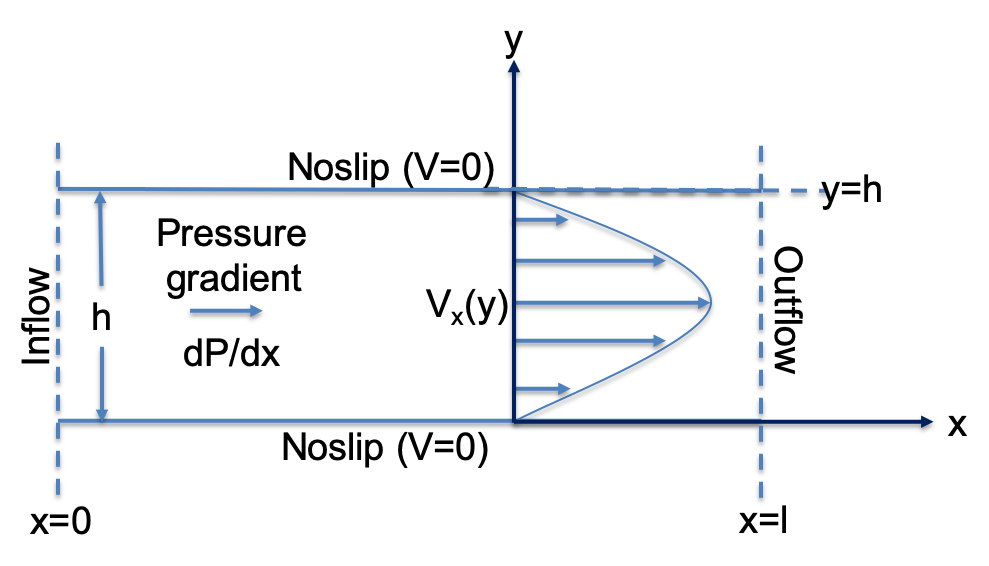
Illustration of the Poiseuille case setup
The exact Poiseuille solution is defined by the following:
\[\begin{split} P(x) &= P_{\text{hi}} + P'x\\ v_x &= \frac{-P'}{2\mu}y(h-y), v_y = 0\\ \rho &= \rho_0\\ \rho{E} &= \frac{P(x)}{(\gamma-1)} + \frac{\rho}{2}(\mathbf{v}\cdot\mathbf{v}) \end{split}\]Here, \(P'\) is the constant slope of the linear pressure gradient from the inlet to the outlet and is calculated as:
\(v_x\), and \(v_y\) are respectively the x and y components of the velocity, \(\mathbf{v}\), and \(\rho_0\) is the supplied constant density of the fluid.\[ P' = \frac{(P_{\text{low}}-P_{\text{hi}})}{\text{length}} \]
- class mirgecom.initializers.ShearFlow(dim=2, mu=0.01, gamma=1.5, density=1.0, flow_dir=0, trans_dir=1)[source]
Shear flow exact Navier-Stokes solution from [Hesthaven_2008].
The shear flow solution is described in Section 7.5.3 of [Hesthaven_2008]. It is generalized to major-axis-aligned 3-dimensional cases here and defined as:
\[\begin{split}\rho &= 1\\ v_\parallel &= r_{t}^2\\ \mathbf{v}_\bot &= 0\\ E &= \frac{2\mu{r_\parallel} + 10}{\gamma-1} + \frac{r_{t}^4}{2}\\ \gamma &= \frac{3}{2}, \mu=0.01, \kappa=0\end{split}\]with fluid total energy \(E\), viscosity \(\mu\), and specific heat ratio \(\gamma\). The flow velocity is \(\mathbf{v}\) with flow speed and direction \(v_\parallel\), and \(r_\parallel\), respectively. The flow velocity in all directions other than \(r_\parallel\), is denoted as \(\mathbf{v}_\bot\). One major-axis-aligned flow-transverse direction, \(r_t\) is set by the user. This shear flow solution is an exact solution to the fully compressible Navier-Stokes equations when neglecting thermal terms; i.e., when thermal conductivity \(\kappa=0\). This solution requires a 2d or 3d domain.
4.4.11. State Initializers
4.4.12. Initialization Utilities
- mirgecom.initializers.make_pulse(amp, r0, w, r)[source]
Create a Gaussian pulse.
The Gaussian pulse is defined by:
\[G(\mathbf{r}) = a_0*\exp^{-(\frac{(\mathbf{r}-\mathbf{r}_0)}{\sqrt{2}w})^{2}},\]where \(\mathbf{r}\) is the position, and the parameters are the pulse amplitude \(a_0\), the pulse location \(\mathbf{r}_0\), and the rms width of the pulse, \(w\).
- Parameters:
amp (float) – specifies the value of \(a_0\), the pulse amplitude
r0 (numpy.ndarray) – specifies the value of \(\mathbf{r}_0\), the pulse location
w (float) – specifies the value of \(w\), the rms pulse width
r (numpy.ndarray) – specifies the nodal coordinates
- Returns:
G – The values of the exponential function
- Return type:
mirgecom.euler helps solve Euler’s equations of gas dynamics.
Euler’s equations of gas dynamics:
where:
state \(\mathbf{Q} = [\rho, \rho{E}, \rho\vec{V}, \rho{Y}_\alpha]\)
flux \(\mathbf{F} = [\rho\vec{V},(\rho{E} + p)\vec{V}, (\rho(\vec{V}\otimes\vec{V}) + p*\mathbf{I}), \rho{Y}_\alpha\vec{V}]\),
unit normal \(\hat{n}\) to the domain boundary \(\partial\Omega\),
vector of species mass fractions \({Y}_\alpha\), with \(1\le\alpha\le\mathtt{nspecies}\).
4.4.13. RHS Evaluation
- mirgecom.euler.euler_operator(dcoll, state, gas_model, boundaries, time=0.0, inviscid_numerical_flux_func=None, quadrature_tag=<class 'grudge.dof_desc.DISCR_TAG_BASE'>, dd=DOFDesc(domain_tag=VolumeDomainTag(tag=<class 'grudge.dof_desc.VTAG_ALL'>), discretization_tag=<class 'grudge.dof_desc.DISCR_TAG_BASE'>), comm_tag=None, use_esdg=False, operator_states_quad=None, entropy_conserving_flux_func=None, limiter_func=None, entropy_min=None)[source]
Compute RHS of the Euler flow equations.
- Returns:
The right-hand-side of the Euler flow equations:
\[\dot{\mathbf{q}} = - \nabla\cdot\mathbf{F} + (\mathbf{F}\cdot\hat{n})_{\partial\Omega}\]- Return type:
- Parameters:
state (
FluidState) – Fluid state object with the conserved state, and dependent quantities.boundaries – Dictionary of boundary functions, one for each valid
BoundaryDomainTagtime – Time
gas_model (
GasModel) – Physical gas model including equation of state, transport, and kinetic properties as required by fluid statequadrature_tag – An optional identifier denoting a particular quadrature discretization to use during operator evaluations.
dd (grudge.dof_desc.DOFDesc) – the DOF descriptor of the discretization on which state lives. Must be a volume on the base discretization.
comm_tag (Hashable) – Tag for distributed communication
4.4.14. Logging Helpers
mirgecom.inviscid provides helper functions for inviscid flow.
4.4.15. Inviscid Flux Calculation
- mirgecom.inviscid.inviscid_flux(state)[source]
Compute the inviscid flux vectors from fluid conserved vars cv.
The inviscid fluxes are \((\rho\vec{V},(\rho{E}+p)\vec{V},\rho(\vec{V}\otimes\vec{V}) +p\mathbf{I}, \rho{Y_s}\vec{V})\)
Note
The fluxes are returned as a
mirgecom.fluid.ConservedVarsobject with a dim-vector for each conservation equation. Seemirgecom.fluid.ConservedVarsfor more information about how the fluxes are represented.- Parameters:
state (
FluidState) – Full fluid conserved and thermal state.- Returns:
A CV object containing the inviscid flux vector for each conservation equation.
- Return type:
- mirgecom.inviscid.inviscid_facial_flux_rusanov(state_pair, gas_model, normal)[source]
High-level interface for inviscid facial flux using Rusanov numerical flux.
The Rusanov or Local Lax-Friedrichs (LLF) inviscid numerical flux is calculated as:
\[F^{*}_{\mathtt{Rusanov}} = \frac{1}{2}(\mathbf{F}(q^-) +\mathbf{F}(q^+)) \cdot \hat{n} + \frac{\lambda}{2}(q^{-} - q^{+}),\]where \(q^-, q^+\) are the fluid solution state on the interior and the exterior of the face where the Rusanov flux is to be calculated, \(\mathbf{F}\) is the inviscid fluid flux, \(\hat{n}\) is the face normal, and \(\lambda\) is the local maximum fluid wavespeed.
- Parameters:
state_pair (
TracePair) – Trace pair ofFluidStatefor the face upon which the flux calculation is to be performedgas_model (
GasModel) – Physical gas model including equation of state, transport, and kinetic properties as required by fluid statenormal (numpy.ndarray) – The element interface normals
- Returns:
A CV object containing the scalar numerical fluxes at the input faces. The returned fluxes are scalar because they’ve already been dotted with the face normals as required by the divergence operator for which they are being computed.
- Return type:
- mirgecom.inviscid.inviscid_facial_flux_hll(state_pair, gas_model, normal)[source]
High-level interface for inviscid facial flux using HLL numerical flux.
The Harten, Lax, van Leer approximate riemann numerical flux is calculated as:
\[f^{*}_{\mathtt{HLL}} = \frac{\left(s^+f^--s^-f^++s^+s^-\left(q^+-q^-\right) \right)}{\left(s^+ - s^-\right)}\]where \(f^{\mp}\), \(q^{\mp}\), and \(s^{\mp}\) are the interface-normal fluxes, the states, and the wavespeeds for the interior (-) and exterior (+) of the interface respectively.
Details about how the parameters and fluxes are calculated can be found in Section 10.3 of [Toro_2009].
- Parameters:
state_pair (
TracePair) – Trace pair ofFluidStatefor the face upon which the flux calculation is to be performedgas_model (
GasModel) – Physical gas model including equation of state, transport, and kinetic properties as required by fluid statenormal (numpy.ndarray) – The element interface normals
- Returns:
A CV object containing the scalar numerical fluxes at the input faces. The returned fluxes are scalar because they’ve already been dotted with the face normals as required by the divergence operator for which they are being computed.
- Return type:
- mirgecom.inviscid.inviscid_flux_on_element_boundary(dcoll, gas_model, boundaries, interior_state_pairs, domain_boundary_states, quadrature_tag=<class 'grudge.dof_desc.DISCR_TAG_BASE'>, numerical_flux_func=<function inviscid_facial_flux_rusanov>, time=0.0, dd=DOFDesc(domain_tag=VolumeDomainTag(tag=<class 'grudge.dof_desc.VTAG_ALL'>), discretization_tag=<class 'grudge.dof_desc.DISCR_TAG_BASE'>))[source]
Compute the inviscid boundary fluxes for the divergence operator.
This routine encapsulates the computation of the inviscid contributions to the boundary fluxes for use by the divergence operator. Its existence is intended to allow multiple operators (e.g. Euler and Navier-Stokes) to perform the computation without duplicating code.
- Parameters:
dcoll (
DiscretizationCollection) – A discretization collection encapsulating the DG elementsgas_model (
GasModel) – The physical model constructs for the gas_modelboundaries – Dictionary of boundary functions, one for each valid
BoundaryDomainTaginterior_state_pairs – A
FluidStateTracePair for each internal face.domain_boundary_states – A dictionary of boundary-restricted
FluidState, keyed by boundary domain tags in boundaries.quadrature_tag – An identifier denoting a particular quadrature discretization to use during operator evaluations.
numerical_flux_func – The numerical flux function to use in computing the boundary flux.
time (float) – Time
dd (grudge.dof_desc.DOFDesc) – the DOF descriptor of the discretization on which the fluid lives. Must be a volume on the base discretization.
- mirgecom.inviscid.entropy_conserving_flux_chandrashekar(gas_model, state_ll, state_rr)[source]
Compute the entropy conservative fluxes from states state_ll and state_rr.
This routine implements the two-point volume flux based on the entropy conserving and kinetic energy preserving two-point flux in equations (4.12 - 4.14) of [Chandrashekar_2013].
- Returns:
A CV object containing the matrix-valued two-point flux vectors for each conservation equation.
- Return type:
- mirgecom.inviscid.entropy_conserving_flux_renac(gas_model, state_ll, state_rr)[source]
Compute the entropy conservative fluxes from states cv_ll and cv_rr.
This routine implements the two-point volume flux based on the entropy conserving and kinetic energy preserving two-point flux in equation (24) of [Renac_2021].
- Returns:
A CV object containing the matrix-valued two-point flux vectors for each conservation equation.
- Return type:
- mirgecom.inviscid.entropy_stable_inviscid_facial_flux(state_pair, gas_model, normal, entropy_conserving_flux_func=None, alpha=None)[source]
Return the entropy stable inviscid numerical flux across a face.
This facial flux routine is “entropy stable” in the sense that it computes the flux average component of the interface fluxes using an entropy conservative two-point flux (e.g.
entropy_conserving_flux_chandrashekar()). Additional dissipation is optionally imposed by penalizing the “jump” of the state across interfaces with strength alpha.- Parameters:
state_pair (
TracePair) – Trace pair ofFluidStatefor the face upon which the flux calculation is to be performedgas_model (
GasModel) – Physical gas model including equation of state, transport, and kinetic properties as required by fluid statenormal (numpy.ndarray) – The element interface normals
entropy_conserving_flux_func – Callable function returning the entropy-conserving flux function to use. If unspecified, an appropriate flux function will be chosen depending on the type of fluid state (e.g. mixture vs. single gas).
alpha – Strength of the penalization term. This can be a fixed single scalar, or a
DOFArray. For example, a Rusanov flux can be constructed by passing the max wavespeed as alpha.
- Returns:
A CV object containing the scalar numerical fluxes at the input faces.
- Return type:
- mirgecom.inviscid.entropy_stable_inviscid_facial_flux_rusanov(state_pair, gas_model, normal, entropy_conserving_flux_func=None, **kwargs)[source]
Return the entropy stable inviscid numerical flux.
This facial flux routine is “entropy stable” in the sense that it computes the flux average component of the interface fluxes using an entropy conservative two-point flux (e.g.
entropy_conserving_flux_chandrashekar()). Rusanov dissipation is imposed by penalizing the “jump” of the state across interfaces with the max wavespeed between the two (+/-) facial states.- Parameters:
state_pair (
TracePair) – Trace pair ofFluidStatefor the face upon which the flux calculation is to be performedgas_model (
GasModel) – Physical gas model including equation of state, transport, and kinetic properties as required by fluid statenormal (numpy.ndarray) – The element interface normals
entropy_conserving_flux_func – Callable function returning the entropy-conserving flux function to use. If unspecified, an appropriate flux function will be chosen depending on the type of fluid state (e.g. mixture vs. single gas).
- Returns:
A CV object containing the scalar numerical fluxes at the input faces.
- Return type:
4.4.16. Inviscid Time Step Computation
- mirgecom.inviscid.get_inviscid_timestep(dcoll, state, dd=DOFDesc(domain_tag=VolumeDomainTag(tag=<class 'grudge.dof_desc.VTAG_ALL'>), discretization_tag=<class 'grudge.dof_desc.DISCR_TAG_BASE'>))[source]
Return node-local stable timestep estimate for an inviscid fluid.
The locally required timestep is computed from the acoustic wavespeed:
\[\delta{t}_l = \frac{\Delta{x}_l}{\left(|\mathbf{v}_f| + c\right)},\]where \(\Delta{x}_l\) is the local mesh spacing (given by
characteristic_lengthscales()), and fluid velocity \(\mathbf{v}_f\), and fluid speed-of-sound \(c\), are defined by local state data.- Parameters:
dcoll (grudge.discretization.DiscretizationCollection) – the discretization collection to use
state (
FluidState) – Full fluid conserved and thermal statedd (grudge.dof_desc.DOFDesc) – the DOF descriptor of the discretization on which state lives. Must be a volume on the base discretization.
- Returns:
class – The maximum stable timestep at each node.
- Return type:
~meshmode.dof_array.DOFArray
- mirgecom.inviscid.get_inviscid_cfl(dcoll, state, dt)[source]
Return node-local CFL based on current state and timestep.
- Parameters:
dcoll (
DiscretizationCollection) – the discretization collection to usedt (float or
DOFArray) – A constant scalar dt or node-local dtstate (
FluidState) – The full fluid conserved and thermal state
- Returns:
The CFL at each node.
- Return type:
mirgecom.viscous provides helper functions for viscous flow.
4.4.17. Viscous Flux Calculation
- mirgecom.viscous.viscous_flux(state, grad_cv, grad_t)[source]
Compute the viscous flux vectors.
The viscous fluxes are:
\[\mathbf{F}_V = [0,\tau\cdot\mathbf{v} - \mathbf{q}, \tau,-\mathbf{J}_\alpha],\]with fluid velocity (\(\mathbf{v}\)), viscous stress tensor (\(\mathbf{\tau}\)), heat flux (\(\mathbf{q}\)), and diffusive flux for each species (\(\mathbf{J}_\alpha\)).
Note
The fluxes are returned as a
mirgecom.fluid.ConservedVarsobject with a dim-vector for each conservation equation. Seemirgecom.fluid.ConservedVarsfor more information about how the fluxes are represented.- Parameters:
state (
FluidState) – Full fluid conserved and thermal stategrad_cv (
ConservedVars) – Gradient of the fluid stategrad_t (numpy.ndarray) – Gradient of the fluid temperature
- Returns:
The viscous transport flux vector if viscous transport properties are provided, scalar zero otherwise.
- Return type:
ConservedVarsor float
- mirgecom.viscous.viscous_stress_tensor(state, grad_cv)[source]
Compute the viscous stress tensor.
The viscous stress tensor \(\tau\) is defined by:
\[\mathbf{\tau} = \mu\left(\nabla{\mathbf{v}} +\left(\nabla{\mathbf{v}}\right)^T\right) + (\mu_B - \frac{2\mu}{3}) \left(\nabla\cdot\mathbf{v}\right)\]- Parameters:
state (
FluidState) – Full conserved and thermal state of fluidgrad_cv (
ConservedVars) – Gradient of the fluid state
- Returns:
The viscous stress tensor
- Return type:
- mirgecom.viscous.diffusive_flux(state, grad_cv)[source]
Compute the species diffusive flux vector, (\(\mathbf{J}_{\alpha}\)).
The species diffusive flux is defined by:
\[\mathbf{J}_{\alpha} = -\rho\left({d}_{(\alpha)}\nabla{Y_{\alpha}} -Y_{(\alpha)}{d}_{\alpha}\nabla{Y_{\alpha}}\right),\]with gas density \(\rho\), species diffusivities \({d}_{\alpha}\), and species mass fractions \({Y}_{\alpha}\). The first term on the RHS is the usual diffusive flux, and the second term is a mass conservation correction term to ensure \(\Sigma\mathbf{J}_\alpha = 0\). The parens \((\alpha)\) indicate no sum over repeated indices is to be performed.
- Parameters:
state (
FluidState) – Full fluid conserved and thermal stategrad_cv (
ConservedVars) – Gradient of the fluid state
- Returns:
The species diffusive flux vector, \(\mathbf{J}_{\alpha}\)
- Return type:
- mirgecom.viscous.conductive_heat_flux(state, grad_t)[source]
Compute the conductive heat flux, (\(\mathbf{q}_{c}\)).
The conductive heat flux is defined by:
\[\mathbf{q}_{c} = -\kappa\nabla{T},\]with thermal conductivity \(\kappa\), and gas temperature \(T\).
- Parameters:
state (
FluidState) – Full fluid conserved and thermal stategrad_t (numpy.ndarray) – Gradient of the fluid temperature
- Returns:
The conductive heat flux vector
- Return type:
- mirgecom.viscous.diffusive_heat_flux(state, j)[source]
Compute the diffusive heat flux, (\(\mathbf{q}_{d}\)).
The diffusive heat flux is defined by:
\[\mathbf{q}_{d} = \sum_{\alpha=1}^{\mathtt{Nspecies}}{h}_{\alpha} \mathbf{J}_{\alpha},\]with species specific enthalpy \({h}_{\alpha}\) and diffusive flux ,\(\mathbf{J}_{\alpha}\).
- Parameters:
state (
FluidState) – Full fluid conserved and thermal statej (numpy.ndarray) – The species diffusive flux vector
- Returns:
The total diffusive heat flux vector
- Return type:
- mirgecom.viscous.viscous_facial_flux_central(dcoll, state_pair, grad_cv_pair, grad_t_pair, gas_model=None)[source]
Return a central facial flux for the divergence operator.
The flux is defined as:
\[f_{\text{face}} = \frac{1}{2}\left(\mathbf{f}_v^+ + \mathbf{f}_v^-\right)\cdot\hat{\mathbf{n}},\]with viscous fluxes (\(\mathbf{f}_v\)), and the outward pointing face normal (\(\hat{\mathbf{n}}\)).
- Parameters:
dcoll (
DiscretizationCollection) – The discretization collection to usegas_model (
GasModel) – The physical model for the gas. Unused for this numerical flux function.state_pair (
TracePair) – Trace pair ofFluidStatewith the full fluid conserved and thermal state on the facesgrad_cv_pair (
TracePair) – Trace pair ofConservedVarswith the gradient of the fluid solution on the facesgrad_t_pair (
TracePair) – Trace pair of temperature gradient on the faces.
- Returns:
The viscous transport flux in the face-normal direction on “all_faces” or local to the sub-discretization depending on local input parameter
- Return type:
- mirgecom.viscous.viscous_facial_flux_harmonic(dcoll, state_pair, grad_cv_pair, grad_t_pair, gas_model=None)[source]
Return a central facial flux w/ harmonic mean coefs for the divergence operator.
The flux is defined as:
\[f_{\text{face}} = \frac{1}{2}\left(\mathbf{f}_v(\tilde{k},\mathbf{q}^+,\ldots^+) + \mathbf{f}_v(\tilde{k},\mathbf{q}^-,\ldots^-)\right) \cdot\hat{\mathbf{n}},\]with viscous fluxes (\(\mathbf{f}_v\)), the outward pointing face normal (\(\hat{\mathbf{n}}\)), and thermal conductivity
\[\tilde{k} = 2\frac{k^- k^+}{k^- + k^+}.\]- Parameters:
dcoll (
DiscretizationCollection) – The discretization collection to usegas_model (
GasModel) – The physical model for the gas. Unused for this numerical flux function.state_pair (
TracePair) – Trace pair ofFluidStatewith the full fluid conserved and thermal state on the facesgrad_cv_pair (
TracePair) – Trace pair ofConservedVarswith the gradient of the fluid solution on the facesgrad_t_pair (
TracePair) – Trace pair of temperature gradient on the faces.
- Returns:
The viscous transport flux in the face-normal direction on “all_faces” or local to the sub-discretization depending on local input parameter
- Return type:
- mirgecom.viscous.viscous_flux_on_element_boundary(dcoll, gas_model, boundaries, interior_state_pairs, domain_boundary_states, grad_cv, interior_grad_cv_pairs, grad_t, interior_grad_t_pairs, quadrature_tag=<class 'grudge.dof_desc.DISCR_TAG_BASE'>, numerical_flux_func=<function viscous_facial_flux_central>, time=0.0, dd=DOFDesc(domain_tag=VolumeDomainTag(tag=<class 'grudge.dof_desc.VTAG_ALL'>), discretization_tag=<class 'grudge.dof_desc.DISCR_TAG_BASE'>))[source]
Compute the viscous boundary fluxes for the divergence operator.
This routine encapsulates the computation of the viscous contributions to the boundary fluxes for use by the divergence operator.
- Parameters:
dcoll (
DiscretizationCollection) – A discretization collection encapsulating the DG elementsgas_model (
GasModel) – The physical model constructs for the gas modelboundaries – Dictionary of boundary functions, one for each valid
BoundaryDomainTaginterior_state_pairs – Trace pairs of
FluidStatefor the interior facesdomain_boundary_states – A dictionary of boundary-restricted
FluidState, keyed by boundary domain tags in boundaries.grad_cv (
ConservedVars) – The gradient of the fluid conserved quantities.interior_grad_cv_pairs – Trace pairs of
ConservedVarsfor the interior facesgrad_t – Object array of
DOFArraywith the components of the gradient of the fluid temperatureinterior_grad_t_pairs – Trace pairs for the temperature gradient on interior faces
quadrature_tag – An identifier denoting a particular quadrature discretization to use during operator evaluations.
numerical_flux_func – The numerical flux function to use in computing the boundary flux.
time (float) – Time
dd (grudge.dof_desc.DOFDesc) – the DOF descriptor of the discretization on which the fluid lives. Must be a volume on the base discretization.
4.4.18. Viscous Time Step Computation
- mirgecom.viscous.get_viscous_timestep(dcoll, state, *, dd=DOFDesc(domain_tag=VolumeDomainTag(tag=<class 'grudge.dof_desc.VTAG_ALL'>), discretization_tag=<class 'grudge.dof_desc.DISCR_TAG_BASE'>))[source]
Routine returns the the node-local maximum stable viscous timestep.
The locally required timestep \(\delta{t}_l\) is calculated from the fluid local wavespeed \(s_f\), fluid viscosity \(\mu\), fluid density \(\rho\), and species diffusivities \(d_\alpha\) as:
\[\delta{t}_l = \frac{\Delta{x}_l}{s_l + \left(\frac{\mu}{\rho} + \mathbf{\text{max}}_\alpha(d_\alpha)\right)\left(\Delta{x}_l\right)^{-1}},\]where \(\Delta{x}_l\) is given by
grudge.dt_utils.characteristic_lengthscales(), and the rest are fluid state-dependent quantities. For non-mixture states, species diffusivities \(d_\alpha=0\).- Parameters:
dcoll (
DiscretizationCollection) – the discretization collection to usestate (
FluidState) – Full fluid conserved and thermal statedd (grudge.dof_desc.DOFDesc) – the DOF descriptor of the discretization on which state lives. Must be a volume on the base discretization.
- Returns:
The maximum stable timestep at each node.
- Return type:
- mirgecom.viscous.get_viscous_cfl(dcoll, dt, state, *, dd=DOFDesc(domain_tag=VolumeDomainTag(tag=<class 'grudge.dof_desc.VTAG_ALL'>), discretization_tag=<class 'grudge.dof_desc.DISCR_TAG_BASE'>))[source]
Calculate and return node-local CFL based on current state and timestep.
- Parameters:
dcoll (
DiscretizationCollection) – the discretization collection to usedt (float or
DOFArray) – A constant scalar dt or node-local dtstate (
FluidState) – The full fluid conserved and thermal statedd (grudge.dof_desc.DOFDesc) – the DOF descriptor of the discretization on which state lives. Must be a volume on the base discretization.
- Returns:
The CFL at each node.
- Return type:
- mirgecom.viscous.get_local_max_species_diffusivity(actx, d_alpha)[source]
Return the maximum species diffusivity at every point.
- Parameters:
actx (
ArrayContext) – Array context to used_alpha (numpy.ndarray) – Species diffusivities
- Returns:
The maximum species diffusivity
- Return type:
Compressible Navier-Stokes equations:
where:
fluid state \(\mathbf{Q} = [\rho, \rho{E}, \rho\mathbf{v}, \rho{Y}_\alpha]\)
with fluid density \(\rho\), flow energy \(E\), velocity \(\mathbf{v}\), and vector of species mass fractions \({Y}_\alpha\), where \(1\le\alpha\le\mathtt{nspecies}\).
inviscid flux \(\mathbf{F}_{I} = [\rho\mathbf{v},(\rho{E} + p)\mathbf{v} ,(\rho(\mathbf{v}\otimes\mathbf{v})+p\mathbf{I}), \rho{Y}_\alpha\mathbf{v}]\)
viscous flux \(\mathbf{F}_V = [0,((\tau\cdot\mathbf{v})-\mathbf{q}),\tau_{:i} ,J_{\alpha}]\)
viscous stress tensor \(\mathbf{\tau} = \mu(\nabla\mathbf{v}+(\nabla\mathbf{v})^T) + (\mu_B - \frac{2}{3}\mu)(\nabla\cdot\mathbf{v})\)
diffusive flux for each species \(J_\alpha = -\rho{D}_{\alpha}\nabla{Y}_{\alpha}\)
- total heat flux \(\mathbf{q}=\mathbf{q}_c+\mathbf{q}_d\), is the sum of:
conductive heat flux \(\mathbf{q}_c = -\kappa\nabla{T}\)
diffusive heat flux \(\mathbf{q}_d = \sum{h_{\alpha} J_{\alpha}}\)
fluid pressure \(p\), temperature \(T\), and species specific enthalpies \(h_\alpha\)
fluid viscosity \(\mu\), bulk viscosity \(\mu_{B}\), fluid heat conductivity \(\kappa\), and species diffusivities \(D_{\alpha}\).
4.4.19. RHS Evaluation
Compute the gradient of the fluid conserved variables.
- Parameters:
state (
FluidState) – Fluid state object with the conserved state, and dependent quantities.boundaries – Dictionary of boundary functions, one for each valid
BoundaryDomainTagtime – Time
gas_model (
GasModel) – Physical gas model including equation of state, transport, and kinetic properties as required by fluid statenumerical_flux_func – Optional callable function to return the numerical flux to be used when computing gradients. Defaults to
num_flux_central.quadrature_tag – An identifier denoting a particular quadrature discretization to use during operator evaluations.
dd (grudge.dof_desc.DOFDesc) – the DOF descriptor of the discretization on which state lives. Must be a volume on the base discretization.
comm_tag (Hashable) – Tag for distributed communication
- Returns:
CV object with vector components representing the gradient of the fluid conserved variables.
- Return type:
Compute the gradient of the fluid temperature.
- Parameters:
state (
FluidState) – Fluid state object with the conserved state, and dependent quantities.boundaries – Dictionary of boundary functions keyed by btags
time – Time
gas_model (
GasModel) – Physical gas model including equation of state, transport, and kinetic properties as required by fluid statenumerical_flux_func – Optional callable function to return the numerical flux to be used when computing gradients. Defaults to
num_flux_central.quadrature_tag – An identifier denoting a particular quadrature discretization to use during operator evaluations.
dd (grudge.dof_desc.DOFDesc) – the DOF descriptor of the discretization on which state lives. Must be a volume on the base discretization.
comm_tag (Hashable) – Tag for distributed communication
- Returns:
Array of
DOFArrayrepresenting the gradient of the fluid temperature.- Return type:
Compute RHS of the Navier-Stokes equations.
- Parameters:
state (
FluidState) – Fluid state object with the conserved state, and dependent quantities.boundaries – Dictionary of boundary functions keyed by btags
time – Time
gas_model (
GasModel) – Physical gas model including equation of state, transport, and kinetic properties as required by fluid stateinviscid_numerical_flux_func – Optional callable function providing the face-normal flux to be used for the divergence of the inviscid transport flux. This defaults to
inviscid_facial_flux_rusanov().viscous_numerical_flux_func – Optional callable function providing the face-normal flux to be used for the divergence of the viscous transport flux. This defaults to
viscous_facial_flux_central().gradient_numerical_flux_func – Optional callable function to return the numerical flux to be used when computing gradients in the Navier-Stokes operator.
return_gradients – Optional boolean (defaults to false) indicating whether to return \(\nabla(\text{CV})\) and \(\nabla(T)\) along with the RHS for the Navier-Stokes equations. Useful for debugging and visualization.
quadrature_tag – An identifier denoting a particular quadrature discretization to use during operator evaluations.
dd (grudge.dof_desc.DOFDesc) – the DOF descriptor of the discretization on which state lives. Must be a volume on the base discretization.
comm_tag (Hashable) – Tag for distributed communication
operator_states_quad – Optional iterable container providing the full fluid states (
FluidState) on the quadrature domain (if any) on each of the volume, internal faces tracepairs (including partition boundaries), and minus side of domain boundary faces. If this data structure is not provided, it will be calculated withmake_operator_fluid_states().grad_cv (
ConservedVars) – Optional CV object containing the gradient of the fluid conserved quantities. If not provided, the operator will calculate it withgrad_cv_operator()grad_t (numpy.ndarray) – Optional array containing the gradient of the fluid temperature. If not provided, the operator will calculate it with
grad_t_operator().inviscid_terms_on – Optional boolean to en/disable inviscid terms in this operator. Defaults to ON (True).
- Returns:
The right-hand-side of the Navier-Stokes equations:
\[\partial_t \mathbf{Q} = \nabla\cdot(\mathbf{F}_V - \mathbf{F}_I)\]- Return type:
mirgecom.boundary provides methods and constructs for boundary treatments.
4.4.20. Boundary Treatment Interfaces
- class mirgecom.boundary.FluidBoundary[source]
Abstract interface to fluid boundary treatment.
- abstractmethod inviscid_divergence_flux(dcoll, dd_bdry, gas_model, state_minus, numerical_flux_func, **kwargs)[source]
Get the inviscid boundary flux for the divergence operator.
This routine returns the facial flux used in the divergence of the inviscid fluid transport flux.
- Parameters:
dcoll (
DiscretizationCollection) – A discretization collection encapsulating the DG elementsstate_minus (
FluidState) – Fluid state object with the conserved state, and dependent quantities for the (-) side of the boundary specified by dd_bdry.dd_bdry – Boundary DOF descriptor (or object convertible to one) indicating which domain boundary to process
gas_model (
GasModel) – Physical gas model including equation of state, transport, and kinetic properties as required by fluid statenumerical_flux_func – Function should return the numerical flux corresponding to the divergence of the inviscid transport flux. This function is typically backed by an approximate Riemann solver, such as
inviscid_facial_flux_rusanov().
- Return type:
- abstractmethod viscous_divergence_flux(dcoll, dd_bdry, gas_model, state_minus, grad_cv_minus, grad_t_minus, numerical_flux_func, **kwargs)[source]
Get the viscous boundary flux for the divergence operator.
This routine returns the facial flux used in the divergence of the viscous fluid transport flux.
- Parameters:
dcoll (
DiscretizationCollection) – A discretization collection encapsulating the DG elementsdd_bdry – Boundary DOF descriptor (or object convertible to one) indicating which domain boundary to process
state_minus (
FluidState) – Fluid state object with the conserved state, and dependent quantities for the (-) side of the boundary specified by dd_bdry.grad_cv_minus (
ConservedVars) – The gradient of the conserved quantities on the (-) side of the boundary specified by dd_bdry.grad_t_minus (numpy.ndarray) – The gradient of the fluid temperature on the (-) side of the boundary specified by dd_bdry.
gas_model (
GasModel) – Physical gas model including equation of state, transport, and kinetic properties as required by fluid statenumerical_flux_func – Function should return the numerical flux corresponding to the divergence of the viscous transport flux. This function is typically backed by a helper, such as
viscous_facial_flux_central().
- Return type:
- abstractmethod cv_gradient_flux(dcoll, dd_bdry, gas_model, state_minus, **kwargs)[source]
Get the boundary flux for the gradient of the fluid conserved variables.
This routine returns the facial flux used by the gradient operator to compute the gradient of the fluid solution on a domain boundary.
- Parameters:
dcoll (
DiscretizationCollection) – A discretization collection encapsulating the DG elementsdd_bdry – Boundary DOF descriptor (or object convertible to one) indicating which domain boundary to process
state_minus (
FluidState) – Fluid state object with the conserved state, and dependent quantities for the (-) side of the boundary specified by dd_bdry.gas_model (
GasModel) – Physical gas model including equation of state, transport, and kinetic properties as required by fluid state
- Return type:
- abstractmethod temperature_gradient_flux(dcoll, dd_bdry, gas_model, state_minus, **kwargs)[source]
Get the boundary flux for the gradient of the fluid temperature.
This method returns the boundary flux to be used by the gradient operator when computing the gradient of the fluid temperature at a domain boundary.
- Parameters:
dcoll (
DiscretizationCollection) – A discretization collection encapsulating the DG elementsdd_bdry – Boundary DOF descriptor (or object convertible to one) indicating which domain boundary to process
state_minus (
FluidState) – Fluid state object with the conserved state, and dependent quantities for the (-) side of the boundary specified by dd_bdry.gas_model (
GasModel) – Physical gas model including equation of state, transport, and kinetic properties as required by fluid state
- Return type:
4.4.21. Boundary Conditions Base Classes
- class mirgecom.boundary.PrescribedFluidBoundary(inviscid_flux_func=None, boundary_state_func=None, temperature_gradient_flux_func=None, boundary_temperature_func=None, cv_gradient_flux_func=None, gradient_numerical_flux_func=None, viscous_flux_func=None, boundary_gradient_cv_func=None, boundary_gradient_temperature_func=None)[source]
Abstract interface to a prescribed fluid boundary treatment.
- __init__(inviscid_flux_func=None, boundary_state_func=None, temperature_gradient_flux_func=None, boundary_temperature_func=None, cv_gradient_flux_func=None, gradient_numerical_flux_func=None, viscous_flux_func=None, boundary_gradient_cv_func=None, boundary_gradient_temperature_func=None)[source]
Initialize the PrescribedFluidBoundary and methods.
- inviscid_divergence_flux(dcoll, dd_bdry, gas_model, state_minus, numerical_flux_func=<function inviscid_facial_flux_rusanov>, **kwargs)[source]
Get the inviscid boundary flux for the divergence operator.
- viscous_divergence_flux(dcoll, dd_bdry, gas_model, state_minus, grad_cv_minus, grad_t_minus, numerical_flux_func=<function viscous_facial_flux_central>, **kwargs)[source]
Get the viscous flux for dd_bdry for use in the divergence operator.
- class mirgecom.boundary.MengaldoBoundaryCondition[source]
Abstract interface to Megaldo fluid boundary treatment.
Mengaldo boundary conditions are those described by [Mengaldo_2014], and with slight mods for flow boundaries from [Poinsot_1992] where noted.
4.4. Base class implementations
- inviscid_divergence_flux(dcoll, dd_bdry, gas_model, state_minus, numerical_flux_func=<function inviscid_facial_flux_rusanov>, **kwargs)[source]
Get the inviscid boundary flux for the divergence operator.
This routine returns the facial flux used in the divergence of the inviscid fluid transport flux. Mengaldo BCs use the approximate Riemann solver specified by the numerical_flux_func to calculate the flux. The boundary implementation must provide the
state_plus()to set the exterior state used in the Riemann solver.- Parameters:
dcoll (
DiscretizationCollection) – A discretization collection encapsulating the DG elementsstate_minus (
FluidState) – Fluid state object with the conserved state, and dependent quantities for the (-) side of the boundary specified by dd_bdry.dd_bdry – Boundary DOF descriptor (or object convertible to one) indicating which domain boundary to process
gas_model (
GasModel) – Physical gas model including equation of state, transport, and kinetic properties as required by fluid statenumerical_flux_func – Function should return the numerical flux corresponding to the divergence of the inviscid transport flux. This function is typically backed by an approximate Riemann solver, such as
inviscid_facial_flux_rusanov().
- Return type:
- viscous_divergence_flux(dcoll, dd_bdry, gas_model, state_minus, grad_cv_minus, grad_t_minus, numerical_flux_func=<function viscous_facial_flux_central>, **kwargs)[source]
Get the viscous boundary flux for the divergence operator.
This routine returns the facial flux used in the divergence of the viscous fluid transport flux, (\(f_v\)). The Mengaldo boundary treatment sends back the face-normal component of the physical viscous flux calculated with the boundary conditions:
\[f_v = F_v\left(\text{CV}_\text{bc}, (\nabla{\text{CV}})_\text{bc}, (\nabla{T})_\text{bc}\right) \cdot \hat{n}\]where \(F_v(.,.,.)\) is the viscous flux function and it is called with the boundary conditions of \(\text{CV}\), \(\nabla\text{CV}\), and temperature gradient.
- Parameters:
dcoll (
DiscretizationCollection) – A discretization collection encapsulating the DG elementsdd_bdry – Boundary DOF descriptor (or object convertible to one) indicating which domain boundary to process
state_minus (
FluidState) – Fluid state object with the conserved state, and dependent quantities for the (-) side of the boundary specified by dd_bdry.grad_cv_minus (
ConservedVars) – The gradient of the conserved quantities on the (-) side of the boundary specified by dd_bdry.grad_t_minus (numpy.ndarray) – The gradient of the fluid temperature on the (-) side of the boundary specified by dd_bdry.
gas_model (
GasModel) – Physical gas model including equation of state, transport, and kinetic properties as required by fluid statenumerical_flux_func – Unused!
- Return type:
- cv_gradient_flux(dcoll, dd_bdry, gas_model, state_minus, **kwargs)[source]
Get the boundary flux for the gradient of the fluid conserved variables.
This routine returns the facial flux used by the gradient operator to compute the gradient of the fluid solution on a domain boundary. The Mengaldo boundary treatment sends back \(\text{CV}_bc~\mathbf{\hat{n}}\).
- Parameters:
dcoll (
DiscretizationCollection) – A discretization collection encapsulating the DG elementsdd_bdry – Boundary DOF descriptor (or object convertible to one) indicating which domain boundary to process
state_minus (
FluidState) – Fluid state object with the conserved state, and dependent quantities for the (-) side of the boundary specified by dd_bdry.gas_model (
GasModel) – Physical gas model including equation of state, transport, and kinetic properties as required by fluid state
- Return type:
- temperature_gradient_flux(dcoll, dd_bdry, gas_model, state_minus, **kwargs)[source]
Get the boundary flux for the gradient of the fluid temperature.
This method returns the boundary flux to be used by the gradient operator when computing the gradient of the fluid temperature at a domain boundary. The Mengaldo boundary treatment sends back \(T_bc~\mathbf{\hat{n}}\).
- Parameters:
dcoll (
DiscretizationCollection) – A discretization collection encapsulating the DG elementsdd_bdry – Boundary DOF descriptor (or object convertible to one) indicating which domain boundary to process
state_minus (
FluidState) – Fluid state object with the conserved state, and dependent quantities for the (-) side of the boundary specified by dd_bdry.gas_model (
GasModel) – Physical gas model including equation of state, transport, and kinetic properties as required by fluid state
- Return type:
4.4. Abstract Mengaldo interface
- abstractmethod state_bc(dcoll, dd_bdry, gas_model, state_minus, **kwargs)[source]
Get the boundary condition on the fluid state.
This routine returns the exact value of the boundary condition of the fluid state. These are the values we want to enforce at the boundary. It is used in the calculation of the gradient of the conserved quantities, and in the calculation of the viscous fluxes.
- Parameters:
dcoll (
DiscretizationCollection) – A discretization collection encapsulating the DG elementsstate_minus (
FluidState) – Fluid state object with the conserved state, and dependent quantities for the (-) side of the boundary specified by dd_bdry.dd_bdry – Boundary DOF descriptor (or object convertible to one) indicating which domain boundary to process
gas_model (
GasModel) – Physical gas model including equation of state, transport, and kinetic properties as required by fluid state
- Return type:
- abstractmethod grad_cv_bc(dcoll, dd_bdry, gas_model, state_minus, grad_cv_minus, normal, **kwargs)[source]
Get the boundary condition on the fluid state.
This routine returns the exact value of the boundary condition of the fluid state. These are the values we want to enforce at the boundary. It is used in the calculation of the gradient of the conserved quantities, and in the calculation of the viscous fluxes.
- Parameters:
state_minus (
FluidState) – Fluid state object with the conserved state, and dependent quantities for the (-) side of the boundary specified by dd_bdry.grad_cv_minus (
ConservedVars) – ConservedVars object with the gradient of the fluid conserved variables on the (-) side of the boundary.normal (numpy.ndarray) – Unit normal vector to the boundary
- Return type:
- abstractmethod temperature_bc(dcoll, dd_bdry, state_minus, **kwargs)[source]
Get boundary contition on the temperature.
This routine returns the temperature boundary condition, \(T_\text{bc}\). This value is used in the calcuation of the temperature gradient, \(\nabla{T}\).
- Parameters:
dcoll (
DiscretizationCollection) – A discretization collection encapsulating the DG elementsdd_bdry – Boundary DOF descriptor (or object convertible to one) indicating which domain boundary to process
state_minus (
FluidState) – Fluid state object with the conserved state, and dependent quantities for the (-) side of the boundary.
- Return type:
- abstractmethod grad_temperature_bc(dcoll, dd_bdry, grad_t_minus, normal, **kwargs)[source]
Get the boundary condition on the temperature gradient.
This routine returns the boundary condition on the gradient of the temperature, \((\nabla{T})_\text{bc}\). This value is used in the calculation of the heat flux.
- Parameters:
dcoll (
DiscretizationCollection) – A discretization collection encapsulating the DG elementsdd_bdry – Boundary DOF descriptor (or object convertible to one) indicating which domain boundary to process
grad_t_minus (numpy.ndarray) – Gradient of the temperature on the (-) side of the boundary.
normal (numpy.ndarray) – Unit normal vector to the boundary
- Return type:
- abstractmethod state_plus(dcoll, dd_bdry, gas_model, state_minus, **kwargs)[source]
Get the boundary state to be used for inviscid fluxes.
This routine returns a boundary state that is designed to be used in an approximate Riemann solver, like HLL, or HLLC.
- Parameters:
dcoll (
DiscretizationCollection) – A discretization collection encapsulating the DG elementsstate_minus (
FluidState) – Fluid state object with the conserved state, and dependent quantities for the (-) side of the boundary specified by dd_bdry.dd_bdry – Boundary DOF descriptor (or object convertible to one) indicating which domain boundary to process
gas_model (
GasModel) – Physical gas model including equation of state, transport, and kinetic properties as required by fluid state
- Return type:
4.4.22. Boundary Conditions
- class mirgecom.boundary.DummyBoundary[source]
Boundary type that assigns boundary-adjacent solution to the boundary.
- inviscid_divergence_flux(dcoll, dd_bdry, gas_model, state_minus, numerical_flux_func=<function inviscid_facial_flux_rusanov>, **kwargs)[source]
Get the inviscid boundary flux for the divergence operator.
- viscous_divergence_flux(dcoll, dd_bdry, gas_model, state_minus, grad_cv_minus, grad_t_minus, numerical_flux_func=<function viscous_facial_flux_central>, **kwargs)[source]
Get the viscous flux for dd_bdry for use in the divergence operator.
- class mirgecom.boundary.FarfieldBoundary(free_stream_pressure, free_stream_velocity, free_stream_temperature, free_stream_mass_fractions=None)[source]
Farfield boundary treatment.
This class implements a farfield boundary as described by [Mengaldo_2014] eqn. 30 and eqn. 42. The boundary condition is implemented as:
\[q^{+} = q_\infty\]and the gradients
\[\nabla q_{bc} = \nabla q^{-}\]- __init__(free_stream_pressure, free_stream_velocity, free_stream_temperature, free_stream_mass_fractions=None)[source]
Initialize the boundary condition object.
- state_plus(dcoll, dd_bdry, gas_model, state_minus, **kwargs)[source]
Get the exterior solution on the boundary.
- temperature_bc(dcoll, dd_bdry, state_minus, **kwargs)[source]
Return farfield temperature for use in grad(temperature).
- class mirgecom.boundary.PressureOutflowBoundary(boundary_pressure=101325)[source]
Outflow boundary treatment with prescribed pressure.
This class implements an outflow boundary as described by [Mengaldo_2014]. The boundary condition is implemented as:
\[ \begin{align}\begin{aligned}\rho^+ &= \rho^-\\\rho\mathbf{Y}^+ &= \rho\mathbf{Y}^-\\\rho\mathbf{V}^+ &= \rho\mathbf{V}^-\end{aligned}\end{align} \]For an ideal gas at super-sonic flow conditions, i.e. when:
\[\rho\mathbf{V} \cdot \hat{\mathbf{n}} \ge c,\]then the pressure is extrapolated from interior points:
\[P^+ = P^-\]Otherwise, if the flow is sub-sonic, then the prescribed boundary pressure, \(P^+\), is used. In both cases, the energy is computed as:
\[\rho{E}^+ = \frac{\left(2~P^+ - P^-\right)}{\left(\gamma-1\right)} + \frac{1}{2}\rho^+\left(\mathbf{V}^+\cdot\mathbf{V}^+\right).\]For mixtures, the pressure is imposed or extrapolated in a similar fashion to the ideal gas case. However, the total energy depends on the temperature to account for the species enthalpy and variable specific heat at constant volume. For super-sonic flows, it is extrapolated from interior points:
\[T^+ = T^-\]while for sub-sonic flows, it is evaluated using ideal gas law
\[T^+ = \frac{P^+}{R_{mix} \rho^+}\]- state_plus(dcoll, dd_bdry, gas_model, state_minus, **kwargs)[source]
Get the exterior solution on the boundary.
This is the partially non-reflective boundary state described by [Mengaldo_2014] eqn. 40 if super-sonic, 41 if sub-sonic.
For super-sonic outflow, the interior flow properties (minus) are extrapolated to the exterior point (plus). For sub-sonic outflow, the pressure is imposed on the external point.
For mixtures, the internal energy is obtained via temperature, which comes from ideal gas law with the mixture-weighted gas constant. For ideal gas, the internal energy is obtained directly from pressure.
- temperature_bc(dcoll, dd_bdry, state_minus, **kwargs)[source]
Get temperature value used in grad(T).
- class mirgecom.boundary.RiemannInflowBoundary(cv, temperature)[source]
Inflow boundary treatment.
This class implements an Riemann invariant inflow boundary condition as described by [Mengaldo_2014].
- state_plus(dcoll, dd_bdry, gas_model, state_minus, **kwargs)[source]
Get the exterior solution on the boundary.
This is the partially non-reflective boundary state described by [Mengaldo_2014] eqn. 40 if super-sonic, 41 if sub-sonic.
- temperature_bc(dcoll, dd_bdry, state_minus, **kwargs)[source]
Get temperature value used in grad(T).
- class mirgecom.boundary.RiemannOutflowBoundary(cv, temperature)[source]
Outflow boundary treatment.
This class implements an Riemann invariant for outflow boundary as described by [Mengaldo_2014]. Note that the “minus” and “plus” are different from the reference to the current Mirge-COM definition.
This boundary condition assume isentropic flow, so the regions where it can be applied are not general. Far-field regions are adequate, but not viscous-dominated regions of the flow (such as a boundary layer).
- state_plus(dcoll, dd_bdry, gas_model, state_minus, **kwargs)[source]
Get the exterior solution on the boundary.
This is the Riemann Invariant Boundary Condition described by [Mengaldo_2014] in eqs. 8 to 18.
- temperature_bc(dcoll, dd_bdry, state_minus, **kwargs)[source]
Get temperature value used in grad(T).
- class mirgecom.boundary.IsothermalSlipWallBoundary(wall_temperature=300)[source]
Isothermal viscous slip wall boundary.
This class implements an isothermal slip wall consistent with the prescription by [Mengaldo_2014].
- temperature_bc(dcoll, dd_bdry, state_minus, **kwargs)[source]
Get temperature value used in grad(T).
- grad_cv_bc(dcoll, dd_bdry, gas_model, state_minus, grad_cv_minus, normal, **kwargs)[source]
Return grad(CV) used in the boundary calculation of viscous flux.
Specify the velocity gradients on the external state to ensure zero energy and momentum flux due to shear stresses.
Gradients of species mass fractions are set to zero in the normal direction to ensure zero flux of species across the boundary.
- class mirgecom.boundary.IsothermalWallBoundary(wall_temperature=300)[source]
Isothermal viscous wall boundary.
This class implements an isothermal no-slip wall consistent with the prescription by [Mengaldo_2014].
- temperature_bc(dcoll, dd_bdry, state_minus, **kwargs)[source]
Get temperature value used in grad(T).
- grad_cv_bc(dcoll, dd_bdry, gas_model, state_minus, grad_cv_minus, normal, **kwargs)[source]
Return grad(CV) to be used in the boundary calculation of viscous flux.
- class mirgecom.boundary.AdiabaticSlipBoundary[source]
Boundary condition implementing inviscid slip boundary.
This class implements an adiabatic slip wall consistent with the prescription by [Mengaldo_2014].
- state_plus(dcoll, dd_bdry, gas_model, state_minus, **kwargs)[source]
Return state with reflected normal-component velocity.
- state_bc(dcoll, dd_bdry, gas_model, state_minus, **kwargs)[source]
Return state with zero normal-component velocity.
- temperature_bc(dcoll, dd_bdry, state_minus, **kwargs)[source]
Return temperature for use in grad(temperature).
- grad_cv_bc(dcoll, dd_bdry, gas_model, state_minus, grad_cv_minus, normal, **kwargs)[source]
Return external grad(CV) used in the boundary calculation of viscous flux.
Specify the velocity gradients on the external state to ensure zero energy and momentum flux due to shear stresses.
Gradients of species mass fractions are set to zero in the normal direction to ensure zero flux of species across the boundary.
- class mirgecom.boundary.AdiabaticNoslipWallBoundary[source]
Adiabatic viscous wall boundary.
This class implements an adiabatic no-slip wall consistent with the prescription by [Mengaldo_2014].
- grad_cv_bc(dcoll, dd_bdry, gas_model, state_minus, grad_cv_minus, normal, **kwargs)[source]
Return grad(CV) to be used in the boundary calculation of viscous flux.
- temperature_bc(dcoll, dd_bdry, state_minus, **kwargs)[source]
Get temperature value used in grad(T).
- state_plus(dcoll, dd_bdry, gas_model, state_minus, **kwargs)[source]
Return state with zero-velocity.
- class mirgecom.boundary.LinearizedOutflowBoundary(free_stream_state=None, free_stream_density=None, free_stream_velocity=None, free_stream_pressure=None, free_stream_species_mass_fractions=None)[source]
Characteristics outflow BCs for linearized Euler equations.
Implement non-reflecting outflow based on characteristic variables for the Euler equations assuming small perturbations based on [Giles_1988]. The implementation assumes an uniform, steady flow in which the Euler equations are linearized about, yielding
\[\frac{\partial U}{\partial t} + A \frac{\partial U}{\partial x} + B \frac{\partial U}{\partial y} = 0\]where U is the vector of perturbation (primitive) variables and the coefficient matrices A and B are constant matrices based on the uniform, steady variables.
Using the linear hyperbolic system theory, this equation can be further simplified by ignoring the y-axis terms (tangent) such that wave propagation occurs only along the x-axis direction (normal). Then, the eigendecomposition results in a orthogonal system where the wave have characteristic directions of propagations and enable the creation of non-reflecting outflow boundaries.
This can also be applied for Navier-Stokes equations in regions where viscous effects are not dominant, such as the far-field.
- __init__(free_stream_state=None, free_stream_density=None, free_stream_velocity=None, free_stream_pressure=None, free_stream_species_mass_fractions=None)[source]
Initialize the BC object.
- temperature_bc(dcoll, dd_bdry, state_minus, **kwargs)[source]
Return temperature for use in grad(temperature).
- class mirgecom.boundary.LinearizedInflowBoundary(free_stream_state=None, free_stream_velocity=None, free_stream_pressure=None, free_stream_density=None, free_stream_species_mass_fractions=None)[source]
Characteristics inflow BCs for linearized Euler equations.
- __init__(free_stream_state=None, free_stream_velocity=None, free_stream_pressure=None, free_stream_density=None, free_stream_species_mass_fractions=None)[source]
Initialize the BC object.
- temperature_bc(dcoll, dd_bdry, state_minus, **kwargs)[source]
Return temperature for use in grad(temperature).
mirgecom.flux provides generic inter-elemental flux routines.
4.4.23. Low-level interfaces
- mirgecom.flux.num_flux_lfr(f_minus_normal, f_plus_normal, q_minus, q_plus, lam)[source]
Compute Lax-Friedrichs/Rusanov flux after [Hesthaven_2008], Section 6.6.
The Lax-Friedrichs/Rusanov flux is calculated as:
\[f_{\text{LFR}}=\frac{1}{2}\left(f^-+f^++\lambda\left(q^--q^+\right)\right)\]where \(f^{\mp}\) and \(q^{\mp}\) are the normal flux components and state components on the interior and the exterior of the face over which the LFR flux is to be calculated. \(\lambda\) is the user-supplied dissipation/penalty coefficient.
The \(\lambda\) parameter is system-specific. Specifically, for the Rusanov flux it is the max eigenvalue of the flux jacobian.
- Parameters:
f_minus_normal – Normal component of physical flux interior to (left of) interface
f_plus_normal – Normal component of physical flux exterior to (right of) interface
q_minus – Physical state on interior of interface
q_plus – Physical state on exterior of interface
lam (
DOFArray) – State jump penalty parameter for dissipation term
- Returns:
object array of
DOFArraywith the Lax-Friedrichs/Rusanov numerical flux.- Return type:
- mirgecom.flux.num_flux_central(f_minus_normal, f_plus_normal)[source]
Central low-level numerical flux.
The central flux is calculated as:
\[f_{\text{central}} = \frac{\left(f^++f^-\right)}{2}\]- Parameters:
f_minus_normal – Normal component of physical flux interior to (left of) interface
f_plus_normal – Normal component of physical flux exterior to (right of) interface
- Returns:
object array of
DOFArraywith the central numerical flux.- Return type:
- mirgecom.flux.num_flux_hll(f_minus_normal, f_plus_normal, q_minus, q_plus, s_minus, s_plus)[source]
HLL low-level numerical flux.
The Harten, Lax, van Leer approximate Riemann numerical flux is calculated as:
\[f^{*}_{\text{HLL}} = \frac{\left(s^+f^--s^-f^++s^+s^-\left(q^+-q^-\right) \right)}{\left(s^+ - s^-\right)}\]where \(f^{\mp}\), \(q^{\mp}\), and \(s^{\mp}\) are the interface-normal fluxes, the states, and the wavespeeds for the interior (-) and exterior (+) of the interface, respectively.
Details about this approximate Riemann solver can be found in Section 10.3 of [Toro_2009].
- Parameters:
f_minus_normal – Normal component of physical flux interior to (left of) interface
f_plus_normal – Normal component of physical flux exterior to (right of) interface
q_minus – Physical state on interior of interface
q_plus – Physical state on exterior of interface
q_minus – Physical state on interior of interface
q_plus – Physical state on exterior of interface
s_minus (
DOFArray) – Interface wave-speed parameter for interior of interfaces_plus (
DOFArray) – Interface wave-speed parameter for exterior of interface
- Returns:
object array of
DOFArraywith the HLL numerical flux.- Return type:
mirgecom.limiter is for limiters and limiter-related constructs.
4.4.24. Field limiter functions
- mirgecom.limiter.bound_preserving_limiter(dcoll, field, mmin=0.0, mmax=None, modify_average=False, dd=None)[source]
Implement a slope limiter for bound-preserving properties.
The implementation is summarized in [Zhang_2011], Sec. 2.3, Eq. 2.9, which uses a linear scaling factor
\[\theta = \min\left( \left| \frac{M - \bar{u}_j}{M_j - \bar{u}_j} \right|, \left| \frac{m - \bar{u}_j}{m_j - \bar{u}_j} \right|, 1 \right)\]to limit the high-order polynomials
\[\tilde{p}_j = \theta (p_j - \bar{u}_j) + \bar{u}_j\]The lower and upper bounds are given by \(m\) and \(M\), respectively, and can be specified by the user. By default, no limiting is performed to the upper bound.
The scheme is conservative since the cell average \(\bar{u}_j\) is not modified in this operation. However, a boolean argument can be invoked to modify the cell average. Negative values may appear when changing polynomial order during execution or any extra interpolation (i.e., changing grids). If these negative values remain during the temporal integration, the current slope limiter will fail to ensure positive values.
- Parameters:
dcoll (
grudge.discretization.DiscretizationCollection) – Grudge discretization with boundaries objectfield (meshmode.dof_array.DOFArray or numpy.ndarray) – A field to limit
mmin (float) – Optional float with the target lower bound. Default to 0.0.
mmax (float) – Optional float with the target upper bound. Default to None.
modify_average (bool) – Flag to avoid modification the cell average. Defaults to False.
dd (grudge.dof_desc.DOFDesc) – The DOF descriptor corresponding to field.
- Returns:
An array container containing the limited field(s).
- Return type:
mirgecom.symbolic_fluid provides symbolic versions of fluid constructs.
4.4.25. Symbolic fluxes
- mirgecom.symbolic_fluid.sym_inviscid_flux(sym_cv, sym_pressure)[source]
Return symbolic expression for inviscid flux.
- mirgecom.symbolic_fluid.sym_viscous_flux(sym_cv, sym_temperature, mu=1, kappa=0, species_diffusivities=None)[source]
Return symbolic version of viscous flux.
- mirgecom.symbolic_fluid.sym_diffusive_flux(sym_cv, species_diffusivities=None)[source]
Symbolic diffusive flux calculator.